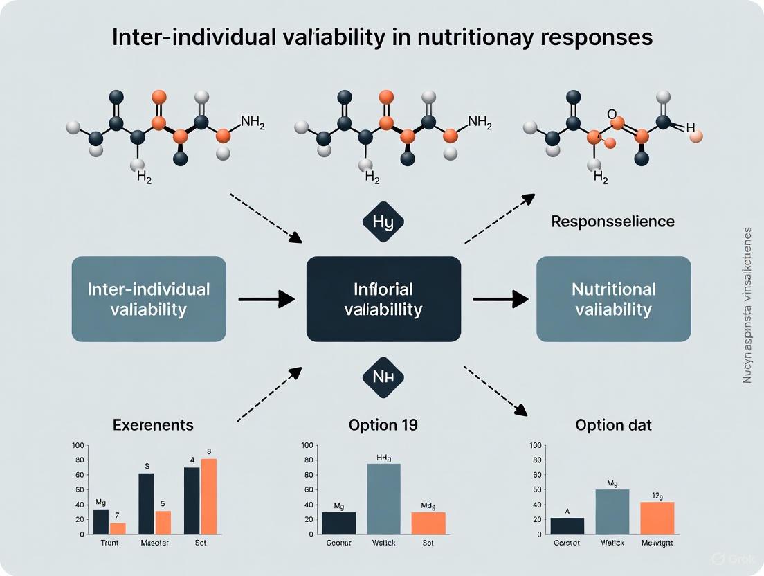
Beyond One-Size-Fits-All: Decoding Inter-Individual Variability in Nutritional Responses for Precision Health
This article provides a comprehensive analysis of inter-individual variability in responses to nutritional interventions, a critical factor often overlooked in traditional diet-related research and drug development.
Beyond One-Size-Fits-All: Decoding Inter-Individual Variability in Nutritional Responses for Precision Health
Abstract
This article provides a comprehensive analysis of inter-individual variability in responses to nutritional interventions, a critical factor often overlooked in traditional diet-related research and drug development. Aimed at researchers, scientists, and drug development professionals, it synthesizes foundational evidence, explores advanced methodological approaches, addresses key challenges in clinical trials, and discusses validation strategies. By integrating insights from recent high-quality studies on topics ranging from dietary nitrate and polyphenols to multi-omics and AI, this review serves as a strategic framework for developing more precise, effective, and personalized nutritional science and therapeutic applications.
The Genetic, Metabolic, and Environmental Roots of Differential Dietary Responses
Core Concepts FAQ
What is inter-individual variability in clinical research? Inter-individual variability (IIV) refers to the differences in how individuals respond to the same intervention, such as a drug, nutrient, or therapy. In clinical trials, this often results in a division between 'responders'—who experience the intended beneficial effect—and 'non-responders'—who experience little to no benefit [1]. This variability is a major challenge for developing universally effective treatments and is a key driver for the move toward personalized or precision medicine.
Why is understanding IIV crucial for nutritional research? In nutritional research, inconsistent findings from randomized controlled trials (RCTs) often stem from significant IIV [2]. For instance, a one-year flavonoid intervention study in postmenopausal women revealed distinct "poor excretors" and "high excretors," which correlated with differences in insulin response [2]. Understanding the sources of this variability is essential to determine for whom a specific nutritional intervention is effective.
What are the primary sources of inter-individual variability? The sources can be categorized into several groups [1]:
- Non-Modifiable Factors: Genetics, sex, and age.
- Modifiable Factors: Gut microbiota composition, health status (e.g., BMI, presence of cardiovascular risk factors), and lifestyle.
- Methodological Factors: Differences in ADME processes (Absorption, Distribution, Metabolism, Excretion) and the responsiveness of cellular and molecular targets.
Is it statistically sound to simply split participants into 'responders' and 'non-responders'? While dichotomization is common, it is often statistically problematic. Converting continuous data (e.g., a 45% improvement) into two categories (responder/non-responder) discards information and generally reduces statistical power [3]. This approach should be reserved for specific cases, such as when outcome distributions are genuinely bimodal (suggesting two distinct populations), and should not be the primary analysis [3].
Troubleshooting Your Research
Problem: High Variability Obscuring Intervention Effects in My Trial
Symptoms:
- Your trial results show a wide standard deviation in the primary outcome measure.
- A subgroup of participants shows a strong positive response, while others show no effect or even a negative response.
- The overall effect in an intention-to-treat (ITT) analysis is statistically non-significant, despite clear anecdotal or subgroup success.
Investigation & Resolution:
| Step | Investigation/Action | Rationale & Methodology |
|---|---|---|
| 1 | Analyze Baseline Data | Conduct post-hoc correlation analyses between participant characteristics (genetics, microbiome, age, sex, health status) and the outcome measure. This can identify potential confounding factors and suggest why effects are seen only in a subgroup [2] [1]. |
| 2 | Conduct Metabotyping | Stratify participants based on their metabolic capacity. Use mass spectrometry-based metabolomic profiling of blood or urine to measure parent compounds and metabolites of the intervention. Group individuals into "metabotypes" (e.g., "producer" vs. "non-producer" of a key bioactive gut metabolite) [2]. |
| 3 | Apply Omics Technologies | Use a multi-omics approach (genomics, metagenomics, transcriptomics) to comprehensively identify factors driving variability. For example, genomics can reveal polymorphisms in genes encoding conjugative enzymes (e.g., UGT1A1, COMT) or transporters that alter the bioavailability of an intervention [2]. |
| 4 | Implement Advanced Statistical Models | Instead of dichotomizing outcomes, use the original continuous data in models that account for bimodality or use machine learning to identify complex, non-linear patterns of response in high-dimensional datasets [2] [3]. |
Problem: Designing a Trial to Actively Capture and Explain IIV
Symptoms:
- Planning a new trial in a field known for high IIV (e.g., polyphenols, exercise cognition, psychiatry).
- The primary goal is to understand which subpopulations benefit from the intervention, not just if it works on average.
Investigation & Resolution:
| Step | Investigation/Action | Rationale & Methodology |
|---|---|---|
| 1 | Enhanced Baseline Assessment | Prior to randomization, collect deep phenotypic data. This should include genetics (e.g., via DNA microarray), gut microbiota (e.g., 16S rRNA or shotgun metagenomic sequencing), detailed health markers, and lifestyle questionnaires [2] [1]. |
| 2 | Choose a Stratified Randomization | Use baseline data (e.g., genetic polymorphisms or microbiome profiles) to stratify participants before randomly assigning them to study arms. This ensures that individuals with distinct metabolic capacities are evenly distributed, allowing for clearer exploration of differential responses [2]. |
| 3 | Select an Adaptive Trial Design | Design the trial to allow for protocol modifications based on interim data analyses. For example, if an interim analysis identifies "responders" and "non-responders," the protocol can be adapted to enrich the study population with a specific subgroup or to adjust the dosage for non-responders [2]. |
| 4 | Consider N-of-1 or Crossover Designs | For short-term interventions, a crossover design, where participants serve as their own control, minimizes the influence of between-subject differences [2]. For a highly personalized approach, N-of-1 trials, where a single participant undergoes multiple cycles of intervention and control, can capture individual response patterns [2]. |
Experimental Protocols & Workflows
Detailed Protocol: Stratifying Participants by Metabotype
Objective: To identify and stratify research participants into "producer" and "non-producer" metabotypes based on their capacity to generate specific microbial metabolites from a polyphenol intervention.
Materials:
- Polyphenol Supplement: Standardized dose (e.g., 500 mg flavanol supplement).
- Collection Tubes: Sterile urine collection containers.
- LC-MS/MS System: Liquid Chromatography with Tandem Mass Spectrometry for high-sensitivity quantification of metabolites.
- Statistical Software: R or Python with packages for multivariate analysis (e.g., PCA, k-means clustering).
Methodology:
- Challenge Test: After an overnight fast, administer a standardized dose of the polyphenol supplement to participants.
- Biospecimen Collection: Collect urine samples at baseline (pre-dose) and at standardized intervals post-administration (e.g., 0-4h, 4-8h, 8-24h). Record exact volumes.
- Sample Preparation: Aliquot urine and process using solid-phase extraction (SPE) to concentrate metabolites and remove salts.
- Metabolomic Profiling: Analyze samples via LC-MS/MS in multiple reaction monitoring (MRM) mode to quantify specific target metabolites known to be produced by the gut microbiota (e.g., γ-valerolactones from flavanols).
- Data Analysis & Stratification:
- Calculate the total urinary excretion of target metabolites over 24 hours.
- Use clustering algorithms (e.g., k-means) on the excretion data to naturally group participants. Typically, two clusters will emerge: "high excretors/producers" and "low excretors/non-producers" [2].
- Validate the clustering stability using statistical methods like bootstrapping.
Investigation Workflow Diagram
Key Determinants of Variability Diagram
The Scientist's Toolkit: Research Reagent Solutions
Essential materials and technologies for investigating inter-individual variability.
| Research Reagent / Technology | Primary Function in IIV Research |
|---|---|
| Standardized Polyphenol Challenge | A uniform, well-characterized dose of a polyphenol (e.g., flavanol pill) used to conduct "challenge tests" that reveal differences in metabolic capacity between individuals [2]. |
| LC-MS/MS (Liquid Chromatography-Tandem Mass Spectrometry) | The gold-standard technology for high-resolution, quantitative metabolomic profiling of polyphenol metabolites in biological fluids like urine and plasma, enabling metabotyping [2]. |
| DNA Microarray / Whole Genome Sequencing | Technologies to identify genetic polymorphisms (e.g., in UGT, SULT, or COMT genes) that are known to influence the metabolism and bioavailability of dietary compounds and drugs [2] [1]. |
| 16S rRNA & Shotgun Metagenomic Sequencing | Methods to characterize the composition and functional potential of the gut microbiome, a major driver of polyphenol metabolism and a key source of IIV [2]. |
| Dynamic Structural Equation Modeling (Dynamic SEM) | An advanced statistical modeling technique used to quantify intraindividual variability from dense, trial-by-trial cognitive or physiological data, separating it from mean performance [4]. |
Frequently Asked Questions (FAQs)
FAQ 1: What is the practical significance of a Genetic Risk Score (GRS) in nutritional research? A Genetic Risk Score (GRS) aggregates the effects of multiple single-nucleotide polymorphisms (SNPs) into a single measure, providing a more powerful tool for assessing an individual's genetic predisposition to complex cardiometabolic traits than single SNPs. It enhances risk prediction even in smaller cohorts and helps explore gene-diet interactions. For example, a GRS based on 18 obesity-related SNPs was significantly associated with higher odds of overweight/obesity, type 2 diabetes (T2DM), and cardiovascular disease (CVD)-related traits. Furthermore, the GRS was the second most predictive factor for BMI after age, demonstrating its utility for risk stratification and personalized nutrition strategies [5].
FAQ 2: Why might my study fail to find a significant association between a GRS and a cardiometabolic trait? Even a well-constructed GRS may not show a direct association with a trait in all study populations. This can occur if the studied population has a unique genetic background, age profile, or is subject to specific environmental modifiers not accounted for in the model. The primary value of a GRS often emerges through its interaction with environmental factors, particularly diet. One study found no direct association between a 39-SNP GRS and cardiometabolic traits but discovered a highly significant interaction between the GRS and carbohydrate intake on HDL-C levels. Always test for gene-diet interactions, as these can reveal the modifying effect of diet on genetic predisposition [6].
FAQ 3: Which genetic variants should I prioritize for constructing a GRS for cardiometabolic traits? SNPs should be selected based on strong prior evidence from genome-wide association studies (GWAS). Focus on variants with established associations to the trait of interest and, crucially, those known to interact with nutrients to provide actionable insights for personalized nutrition. Key genes often include:
- Obesity and Energy Balance:
FTO(rs9939609),MC4R(rs17782313) - Lipid Metabolism:
APOE(rs429358, rs7412),APOC3(rs5128),LIPC(rs1800588) - Glucose Metabolism and T2DM:
TCF7L2(rs7903146, rs12255372) - Other Metabolic Pathways:
ADRB2(rs1042713),CLOCK(rs1801260) [5] [7] [8].
FAQ 4: How do I analyze and interpret a significant gene-diet interaction?
When a significant interaction is detected (e.g., Pinteraction < 0.05), the next step is to perform stratified analysis. This involves examining the relationship between the genetic factor (e.g., GRS) and the outcome (e.g., HDL-C) within different levels of the dietary factor (e.g., tertiles of carbohydrate intake). For instance, research showed that in the highest tertile of carbohydrate intake (>452 g/day), individuals with a high GRS had significantly lower HDL-C, while in the lowest carbohydrate intake tertile, the relationship was reversed. This indicates that the genetic effect is dependent on (or "moderated by") the dietary exposure [6].
FAQ 5: What are the common pitfalls in defining phenotypes and covariates in nutrigenetic studies? Inconsistent or inaccurate phenotyping is a major source of error.
- Phenotypes: Use standardized, objective measures where possible. For obesity, use measured BMI (categorized as normal weight <25 kg/m², overweight/obese ≥25 kg/m²). For T2DM and CVD, combine self-reported medical history with medication use for greater accuracy [5].
- Covariates: Always adjust for key confounding variables such as age, sex, and total energy intake. For population structure, consider genetic principal components or ensuring ethnic homogeneity in your cohort [5] [6].
FAQ 6: How is the field moving beyond traditional GRS approaches? The field is evolving towards multi-omics integration. This involves combining genomic data with other layers of biological information, such as the metabolome, proteome, and gut microbiome, to build more comprehensive predictive models. Machine learning and artificial intelligence (AI) are being employed to analyze these complex datasets, with some models achieving over 90% accuracy in predicting individual metabolic responses to diet. Digital health technologies, like continuous glucose monitors (CGMs), provide real-time phenotypic data that can be correlated with genetic predispositions for dynamic dietary adjustments [9] [10].
Experimental Protocols & Troubleshooting
Protocol: Constructing and Applying a Genetic Risk Score (GRS)
This protocol outlines the steps for creating a GRS from a set of pre-selected SNPs and using it to analyze associations and interactions with cardiometabolic traits [5] [6].
Workflow Overview: The following diagram illustrates the key stages of GRS construction and analysis.
Materials & Reagents:
- Biological Samples: DNA extracted from whole blood, saliva, or buccal swabs [5] [11].
- Genotyping Platform: Microarray or sequencing-based system.
- Software: PLINK, R, or Python for genetic data handling and statistical analysis.
Step-by-Step Procedure:
- SNP Selection & Genotyping:
Quality Control (QC):
GRS Calculation:
- Code each SNP for the number of effect alleles (0, 1, 2).
- Calculate the raw GRS by summing the effect alleles across all SNPs for each individual.
GRS = SNP1 + SNP2 + ... + SNPn[5].
GRS Categorization:
Statistical Analysis:
- Association Test: Use logistic or linear regression to test the association between the GRS (continuous or categorical) and the cardiometabolic trait, adjusting for covariates like age, sex, and principal components of genetic ancestry.
- Example:
log(Trait) ~ GRS + Age + Sex + PC1 + PC2[5].
- Example:
- Interaction Test: To test for a gene-diet interaction, include an interaction term between the GRS and the dietary variable (e.g., carbohydrate intake) in the model.
- Example:
Trait ~ GRS + Carbohydrate_Intake + GRS*Carbohydrate_Intake + Age + Sex[6]. - A significant p-value for the interaction term (
Pinteraction) indicates that the effect of the GRS on the trait depends on the level of carbohydrate intake.
- Example:
- Association Test: Use logistic or linear regression to test the association between the GRS (continuous or categorical) and the cardiometabolic trait, adjusting for covariates like age, sex, and principal components of genetic ancestry.
Troubleshooting Guide:
| Problem | Possible Cause | Solution |
|---|---|---|
| No association between GRS and trait | Population-specific genetic effects; strong environmental modifiers. | Test for gene-environment interactions; validate SNP selection in your population. |
| Low predictive power (AUC) | GRS does not capture sufficient genetic variance. | Increase the number of SNPs in the GRS; consider weighted GRS based on effect sizes from larger GWAS. |
| Significant interaction, but stratified effects are counterintuitive | The relationship is non-linear or confounded. | Visually inspect the interaction plot; ensure dietary intake is accurately measured and adjusted for total energy. |
Protocol: Analyzing Gene-Diet Interactions on Lipid Traits
This protocol provides a detailed methodology for investigating how a GRS and carbohydrate intake interact to influence High-Density Lipoprotein Cholesterol (HDL-C) levels, based on a published study [6].
Workflow Overview: The diagram below outlines the core analytical process for a gene-diet interaction study.
Materials & Reagents:
- Phenotypic Data:
- Outcome: Fasting serum HDL-C (mmol/L).
- Exposures: Genotype data for GRS construction; dietary intake data from a validated Food Frequency Questionnaire (FFQ) or multiple 24-hour recalls.
- Software: Statistical packages like R (preferred) or SPSS.
Step-by-Step Procedure:
- Data Preparation:
- Construct your GRS as described in the previous protocol.
- Process dietary data to derive total daily carbohydrate intake (g/day) and other nutrients of interest (e.g., glycaemic load).
Variable Categorization:
Statistical Modeling:
- Use a linear regression model to test the interaction.
HDL-C ~ GRS_Group + Carb_Tertile + GRS_Group*Carb_Tertile + Age + Sex + Total_Energy_Intake + other_covariates- The key term is
GRS_Group*Carb_Tertile. A significant p-value (Pinteraction) for this term indicates a statistically significant interaction.
Stratified Analysis and Interpretation:
- If the interaction is significant, run separate models within each tertile of carbohydrate intake to understand the direction of the effect.
- Example Result: "In the high-carbohydrate tertile (T3), individuals with a high GRS had a significantly lower HDL-C (Beta = -0.04 mmol/L, p=0.027) compared to those with a low GRS. This effect was not observed in the low-carbohydrate tertile (T1)" [6].
- This suggests that a high-carbohydrate diet is particularly detrimental for HDL-C levels in genetically susceptible individuals.
Troubleshooting Guide:
| Problem | Possible Cause | Solution |
|---|---|---|
| Dietary data is noisy | Recall bias in FFQs; day-to-day variation. | Use the average of multiple 24-hour recalls if possible; adjust for total energy intake to account for reporting errors. |
| Interaction is not significant | Lack of statistical power; incorrect dietary component. | Conduct a power analysis beforehand; explore interactions with other dietary factors (e.g., fat quality, glycaemic index) suggested by literature [7]. |
| Confounding by population stratification | Systematic differences in ancestry and diet. | Adjust for genetic principal components in your models to control for this confounding. |
Data Presentation: Key Gene-Diet Interactions in Cardiometabolic Health
Table 1: Selected Genetic Variants with Evidence for Gene-Diet Interactions
| Gene | SNP (example) | Associated Trait | Interacting Nutrient | Interaction Effect |
|---|---|---|---|---|
| FTO | rs9939609 | Obesity, T2DM | Sugar-Sweetened Beverages (SSBs) | SSB consumption exacerbates obesity risk in risk allele carriers [12]. |
| FTO | rs9939609 | Obesity, T2DM | Physical Activity / Wine | Physical activity and moderate wine consumption attenuate the genetic risk of obesity [12]. |
| MC4R | rs12970134 | Metabolic Syndrome | Dietary Fat | High fat intake increases the risk of MetS in risk allele carriers [7]. |
| APOE | rs429358, rs7412 | LDL-C, CVD Risk | Dietary Saturated Fat | High saturated fat intake has a more adverse effect on LDL-C in carriers of the E4 allele [8]. |
| TCF7L2 | rs7903146 | T2DM, Glucose Metabolism | Dietary Carbohydrate | Risk allele carriers may have a worse glycemic response to high-carbohydrate diets [5] [9]. |
| CLOCK | rs1801260 | Metabolic Syndrome | Dietary Fat | High fat intake interacts with this SNP to increase MetS risk [7]. |
| GRS (Composite) | Multiple | HDL-C | Carbohydrate Intake, Glycaemic Load | High carbohydrate intake/glycaemic load is associated with lower HDL-C specifically in individuals with a high GRS [6]. |
The Scientist's Toolkit: Research Reagent Solutions
Table 2: Essential Materials for Nutrigenetics Experiments
| Item | Function / Application in Research | Example / Note |
|---|---|---|
| DNA Collection Kits | Non-invasive collection of buccal cells or saliva for DNA extraction. Essential for direct-to-consumer and large-scale studies. | Buccal swabs are popular for their convenience and cost-effectiveness [11]. |
| Genotyping Microarrays | High-throughput profiling of hundreds of thousands to millions of SNPs across the genome. | Used in GWAS and for constructing GRS. Platforms from Illumina or Thermo Fisher. |
| Food Frequency Questionnaire (FFQ) | A validated tool to assess habitual dietary intake over a specific period. | Must be validated for the specific population under study (e.g., SONGS project used a 139-item FFQ) [6]. |
| Continuous Glucose Monitor (CGM) | A digital health device that measures interstitial glucose levels in real-time. Provides dense phenotypic data on metabolic response. | Can be used to correlate genetic predisposition with actual glycemic variability in response to meals [9]. |
| Statistical Software (R/Python) | For genetic data QC, GRS calculation, and performing association and interaction regression analyses. | R packages like tidyverse, plyr, and stats are fundamental. PLINK is essential for genetic data handling. |
In nutritional responses research, a significant challenge confounding study outcomes is the substantial inter-individual variability (IIV) in how individuals process dietary compounds. This variation often stems from differences in gut microbiome composition and function, which act as a central metabolic organ. The gut microbiota produces a diverse array of bioactive metabolites from dietary precursors, influencing host physiology in ways that are highly personalized. Understanding these metabotypes—distinct, stable metabolic phenotypes driven by microbial activity—is crucial for designing robust experiments and interpreting variable results. This technical support center provides troubleshooting guides and FAQs to help researchers address these challenges in their experimental workflows.
Frequently Asked Questions (FAQs)
FAQ 1: What are the primary factors driving inter-individual variability in the metabolism of dietary compounds like polyphenols?
Inter-individual variability is primarily driven by an individual's unique gut microbiome composition and activity, which can far exceed the influence of host genetics or diet alone in determining the metabolic fate of many dietary compounds [13] [14] [15]. Other contributing factors include:
- Genetic polymorphisms in host enzymes involved in compound metabolism (e.g., for flavanones and flavan-3-ols) [13].
- Age, sex, ethnicity, and BMI [13].
- Pathophysiological status and physical activity [13].
Two major types of IIV are observed:
- Quantitative Gradients: Individuals can be classified as high or low excretors of specific metabolites [13].
- Qualitative Clusters: Individuals can be clustered as producers versus non-producers of certain metabolites (e.g., equol from isoflavones, urolithins from ellagitannins) [13].
FAQ 2: How significant can inter-individual variation in metabolite production be?
The variation can be substantial. For example, in a study on coffee phenolic acids, the amounts of key microbial metabolites in urine after coffee consumption showed inter-individual variations spanning a 7.5- to 36.3-fold range between the lowest and highest excretors [14]. This highlights that without accounting for metabotypes, group averages can be highly misleading.
FAQ 3: What proportion of the plasma metabolome is explained by the gut microbiome compared to diet and genetics?
A large-scale study quantified the dominant factors for 1,183 plasma metabolites, classifying them as follows [15]:
- 610 metabolites were diet-dominant.
- 85 metabolites were microbiome-dominant.
- 38 metabolites were genetics-dominant.
Collectively, the gut microbiome explained 12.8% of the inter-individual variation in the whole plasma metabolome profile, which was a greater proportion than that explained by genetics (3.3%) though less than that explained by diet (9.3%) [15].
FAQ 4: What are some key bioactive metabolites produced by the gut microbiota?
The gut microbiota produces a wide array of bioactive molecules. The table below summarizes the major classes, their typical compounds, and primary functions [16].
Table 1: Key Bioactive Metabolites from the Gut Microbiota
| Metabolite Class | Typical Metabolites | Primary Functions & Impacts |
|---|---|---|
| Short-Chain Fatty Acids (SCFAs) | Acetate, Propionate, Butyrate | Energy source for colonocytes; regulate gut barrier integrity, immune response, and energy homeostasis [16]. |
| Bile Acids | Deoxycholate, Lithocholate | Facilitate lipid absorption; regulate glucose and lipid metabolism; act as signaling molecules [16]. |
| Tryptophan/Indole Derivatives | Indole, Indole-3-lactic acid, Serotonin | Regulate intestinal barrier function, immune response, and gut motility [16]. |
| Choline Metabolites | Trimethylamine (TMA) | Can promote inflammation and thrombosis; linked to cardiovascular risks [16]. |
| Gases | Hydrogen Sulfide (H₂S), Methane (CH₄) | Regulate gut inflammation, motility, and mucosal blood flow [16]. |
| Neurotransmitters | GABA, Dopamine, Serotonin | Regulate gut motility, memory, stress responses, and immune function [16]. |
Troubleshooting Guides
Problem 1: High Inter-Individual Variation Obscuring Dietary Intervention Effects
Identifying the Cause:
- Symptom: Large standard deviations in endpoint metabolite measurements, lack of statistical significance for a dietary intervention in a cohort, or a bimodal distribution in response data.
- Root Cause: The most likely cause is unaccounted-for inter-individual variation stemming from differences in participants' gut microbiome metabotypes [13] [14]. For instance, you may have a mix of "producers" and "non-producers" for a key microbial metabolite in your study group.
Solution and Experimental Adjustments:
- Pre-Screen and Stratify Participants: Prior to the main intervention, conduct a metabotype screening test. For example, give participants a precursor compound (e.g., daidzein for equol producers, ellagitannins for urolithin producers) and measure the relevant microbial metabolites in urine or blood over 24-48 hours. Stratify your study groups based on producer status (e.g., equol producers vs. non-producers) [13].
- Increase Sample Size: To ensure sufficient statistical power when metabotypes are present but not stratified for, a larger sample size may be required to detect a significant effect within and between metabotype groups.
- Report by Metabotype: If pre-screening is not feasible, analyze and report your results stratified by the metabotype identified during the study, rather than only reporting the group mean. This provides a more accurate picture of the intervention's effect [13].
Problem 2: Inconsistent Metabolomic Profiles in Urine Samples
Identifying the Cause:
- Symptom: High intra- and inter-individual variability in untargeted metabolomic analysis of urine, making it difficult to distinguish dietary signals from background noise.
- Root Cause: Uncontrolled factors such as the timing of the last meal, fluid intake, physical activity, and the absence of a standardized pre-sampling protocol can dramatically alter the urine metabolome [17].
Solution and Protocol Implementation: Adopt a standardized protocol for sample collection to minimize confounding variability [17].
- Standardize the Evening Meal: Provide participants with a standardized, metabolically "neutral" evening meal low in plant polyphenols and specific bioactive compounds the night before sampling [17].
- Control Fasting and Fluid Intake: Enforce a consistent overnight fast (e.g., 12 hours) and control water intake before sample collection. Record the volume of water consumed [17].
- Define Collection Timing:
- Collect a fasting urine sample upon arrival at the clinic as a stable baseline.
- Collect postprandial samples within a consistent time window (e.g., 2-4 hours after a standardized test meal), as the urine composition has been shown to be stable during this period [17].
- Pooled overnight urine can also serve as a useful baseline [17].
- Use Normalization Factors: Apply normalization to metabolomic data to account for dilution, such as using urine volume, osmolarity, or creatinine levels [17].
Problem 3: Failed Discovery of Novel Microbial Metabolites
Identifying the Cause:
- Symptom: Inability to detect or identify novel bioactive non-peptide metabolites from microbial cultures or fecal samples.
- Root Cause: Reliance on traditional culture-dependent methods that miss uncultured species, or use of analytical methods not optimized for the chemical diversity of microbial metabolites [18].
Solution and Workflow Optimization:
- Employ Culture-Independent Methods: Utilize metagenomic sequencing to identify biosynthetic gene clusters (BGCs) in the gut microbiome that code for novel metabolites. Tools like antiSMASH and PRISM can be used for this prediction [18].
- Apply Advanced Metabolomics:
- Use untargeted metabolomics with complementary liquid chromatography/mass spectrometry (LC/MS) methods to maximize coverage [19].
- For hydrophilic metabolites (e.g., many microbial fermentation products), use Hydrophilic Interaction Liquid Chromatography (HILIC) coupled to a high-resolution accurate mass instrument (e.g., Orbitrap) [19].
- Include stable isotope-labeled internal standards (e.g., l-Phenylalanine-d8, l-Valine-d8) for quality control during sample extraction and analysis [19].
Experimental Protocols
Detailed Protocol: Untargeted Metabolomic Analysis of Biofluids Using HILIC-MS
This protocol is adapted for analyzing polar microbial metabolites (e.g., SCFAs, organic acids) in plasma, urine, or fecal water [19].
1. Sample Preparation and Extraction:
- Prepare an extraction solvent of acetonitrile:methanol:formic acid (74.9:24.9:0.2, v/v/v) [19].
- For example, mix 100 µL of biofluid (e.g., plasma, urine) with 300 µL of ice-cold extraction solvent containing internal standards.
- Vortex vigorously, then centrifuge at high speed (e.g., 14,000-16,000 x g) for 10-15 minutes at 4°C.
- Transfer the clear supernatant to a new vial for LC-MS analysis.
2. Liquid Chromatography (HILIC Separation):
- Column: Use a HILIC column (e.g., Waters Atlantis HILIC Silica, 3 µm, 2.1 x 150 mm) [19].
- Mobile Phase A: 10 mM ammonium formate with 0.1% formic acid in water [19].
- Mobile Phase B: 0.1% formic acid in acetonitrile [19].
- Gradient: Use a gradient elution, for example:
- Start at 85% B.
- Ramp to 40% B over 10-15 minutes.
- Hold for 2-3 minutes.
- Re-equilibrate to 85% B for 5-7 minutes.
- Flow Rate: 0.3-0.4 mL/min.
- Column Temperature: 30-40°C.
- Injection Volume: 5-10 µL.
3. Mass Spectrometry (Orbitrap Detection):
- Ionization: Electrospray Ionization (ESI) in both positive and negative modes.
- Resolution: Set to high resolution (e.g., >60,000 at m/z 200).
- Mass Range: m/z 70-1000.
- Data Acquisition: Full-scan MS mode for untargeted profiling.
4. Data Processing:
- Use software (e.g., Thermo Compound Discoverer, XCMS, MS-DIAL) for peak picking, alignment, and compound identification by matching to online databases (e.g., HMDB, MassBank).
Research Reagent Solutions
Table 2: Essential Materials for Gut Microbiome and Metabolomics Research
| Item | Function/Application | Example/Note |
|---|---|---|
| HILIC LC Column | Separation of polar metabolites in untargeted metabolomics. | Waters Atlantis HILIC Silica column [19]. |
| High-Resolution Mass Spectrometer | Accurate mass detection and identification of metabolites. | Orbitrap mass spectrometer [19]. |
| Stable Isotope-Labeled Internal Standards | Quality control for sample extraction and instrument performance; semi-quantification. | l-Phenylalanine-d8, l-Valine-d8 [19]. |
| Standardized Test Meals | Control dietary input to reduce background variability in nutritional studies. | Meals low in target polyphenols for pre-study standardization [17]. |
| Biosynthetic Gene Cluster (BGC) Prediction Software | In silico identification of potential microbial metabolite pathways from genomic data. | antiSMASH, PRISM4 [18]. |
Visualizations: Pathways and Workflows
Diagram: Gut Microbiome's Role in Metabolic Variability
Diagram: Experimental Protocol for Robust Nutritional Metabolomics
Frequently Asked Questions (FAQs)
FAQ 1: Why do participants in my nutritional study respond so differently to the same dietary intervention? Inter-individual variation in response to diet is a well-recognized phenomenon driven by multiple intrinsic factors. These include differences in genetic background (such as polymorphisms affecting nutrient metabolism), gut microbiome composition and function, sex, age, and circadian rhythms [20] [21]. These factors influence the absorption, metabolism, distribution, and bioavailability of nutrients, leading to a wide range of physiological responses even under highly controlled conditions [22] [21].
FAQ 2: How do age and sex specifically influence circadian rhythms and subsequent metabolic responses? Research shows clear demographic differences in circadian physiology. Sex differences exist, with women often exhibiting higher vagal oscillatory activity and more stable circadian rhythms than men [23] [24]. Aging is associated with chronodisruption, characterized by dampened circadian rhythms, earlier timing of peak activity (acrophase), and reduced overall variability in cardiac autonomic markers [23] [25]. These differences in internal timekeeping can modify metabolic responses to food intake timed at different circadian phases [25].
FAQ 3: What is the evidence that inter-individual differences in appetitive sensations are stable over time? Observational studies have demonstrated that sensations like hunger, fullness, and thirst show marked and stable inter-individual differences over periods as long as 17 weeks. High correlation coefficients for these sensations (e.g., r=0.67 to 0.88 for thirst) across multiple weeks confirm that an individual's baseline appetite profile is a consistent trait-like factor that should be accounted for in study design [26].
FAQ 4: Can we predict who will respond to a specific nutritional intervention? Current research is actively exploring this question using multi-omics approaches. While studies have attempted to use metabolomic profiles to distinguish responders from non-responders, success has been limited. For example, a blueberry intervention found extensive inter-individual variation in vascular and cognitive endpoints but could not identify a consistent predictive urinary metabolite [21]. This remains a primary challenge and goal for precision nutrition.
FAQ 5: How can controlled feeding studies be designed to better account for this variability? Controlled feeding studies, particularly with randomized crossover designs, are ideal for testing genotype-diet and phenotype-diet interactions because each participant serves as their own control [20]. Participant screening can be designed to a priori enrich for specific genotypes or phenotypes to ensure balanced subgroup sample sizes and increase statistical power for comparing these subgroups [20].
Troubleshooting Common Experimental Issues
Problem: High Unexplained Variance in Primary Endpoints
- Potential Cause: Unaccounted for demographic and physiological modifiers such as circadian timing of assessments, participant sex, or age-related metabolic differences.
- Solution:
- Stratify Recruitment: Recruit participants stratified by sex and age groups rather than treating them as homogeneous groups [23] [26].
- Standardize Timing: Conduct all assessments and interventions at a fixed clock time relative to the participant's wake-up time to control for circadian phase. Record the time of data collection for use as a covariate in statistical models [23] [25].
- Measure, Don't Assume: Collect baseline data on key modifiers (e.g., chronotype via questionnaires, appetitive sensations) instead of relying on population averages [26] [24].
Problem: Inconsistent Replication of Dietary Intervention Effects
- Potential Cause: Inter-individual variation in gut microbiome capacity to metabolize specific dietary components (e.g., polyphenols, fibers) into active compounds [20] [21].
- Solution:
- Profile Baseline Microbiome: Collect and sequence fecal samples at baseline to characterize the gut microbiome as a potential source of variation [20].
- Include Metabolomics: Integrate targeted metabolomic profiling of blood or urine to measure bioactive metabolites and account for differences in microbial metabolism [21].
- Consider Genotyping: For nutrients with known metabolism pathways (e.g., catechols), genotype participants for relevant polymorphisms (e.g., COMT)[ccitation:10].
Table 1: Impact of Sex and Age on Circadian Cardiac Autonomic Parameters (via Heart Rate Variability Analysis)
| Parameter | Sex Effect (Women vs. Men) | Aging Effect (Older vs. Younger) |
|---|---|---|
| Overall Vagal Activity | Higher oscillatory activity [23] | Diminished fluctuations [23] |
| Circadian Rhythm Stability | More stable rhythms (higher interdaily stability) [24] | Variable findings; can be more stable but also more fragmented [23] [24] |
| Circadian Rhythm Fragmentation | Less fragmented rhythms (lower interdaily variability) [24] | Increased fragmentation [23] |
Table 2: Stability of Self-Reported Appetitive Sensations Over 17 Weeks (Pearson's r)
| Sensation | Week 1 vs. Week 9 | Week 1 vs. Week 17 | Week 9 vs. Week 17 |
|---|---|---|---|
| Hunger | 0.72 [26] | 0.67 [26] | 0.77 [26] |
| Fullness | 0.74 [26] | 0.71 [26] | 0.81 [26] |
| Thirst | 0.82 [26] | 0.81 [26] | 0.88 [26] |
Table 3: Range of Inter-individual Response to a One-Week Blueberry Intervention
| Endpoint Category | Specific Parameter | Observed Range of Response (% Change from Baseline) |
|---|---|---|
| Vascular Health | Not Specified | -141% to +525% [21] |
| Cognitive Function | Not Specified | -114% to +96% [21] |
Detailed Experimental Protocols
Protocol 1: Assessing Stable Inter-Individual Differences in Appetitive Sensations [26] This protocol outlines a method to establish baseline trait-level appetitive sensations in study participants.
- Participant Training: Conduct appetite lexicon training using standardized videos defining hunger, fullness, desire to eat, and prospective consumption. Administer a quiz requiring a ≥90% pass rate to ensure concept understanding.
- Study Design: Implement a longitudinal observational study with data collection at multiple timepoints (e.g., weeks 1, 9, and 17).
- Data Collection:
- On each assessment day (e.g., 2 weekdays + 1 weekend day per timepoint), participants rate hunger, fullness, and thirst hourly during waking hours using a 100 mm Visual Analog Scale (VAS) on an electronic survey.
- Enforce compliance via time/date stamps with an acceptance window of ±5 minutes.
- Simultaneously, collect 24-hour dietary intake data using a validated automated self-administered recall system (e.g., ASA24) and physical activity data via a pedometer app.
- Data Analysis:
- Calculate the daily mean for each appetitive sensation.
- Use one-way ANOVA to investigate within- and between-individual variances.
- Assess temporal stability by calculating Pearson's correlation coefficients between the mean ratings from different weeks.
Protocol 2: Characterizing Inter-Individual Variability in Response to a Blueberry Intervention [21] This protocol describes a method to quantify and analyze differential responses to a controlled dietary intervention.
- Study Design: A single-blinded, crossover, randomized controlled trial (RCT) with three arms: whole fruit, freeze-dried powder, and a placebo control, each administered for one week with a one-week washout period.
- Participant Preparation: Provide participants with a list of polyphenol-rich foods and dietary nitrates/nitrites to avoid for the duration of the study. Collect food diaries to monitor compliance.
- Endpoint Measurement: Measure a battery of endpoints pre- and post-intervention.
- Vascular Function: Systolic and diastolic blood pressure (3 readings each), carotid-radial pulse wave velocity (PWV), plasma glucose, nitrite, and cholesterol levels.
- Cognitive Function: Assess memory and executive function using standardized cognitive tests.
- Metabolomics: Collect urine samples for non-targeted metabolomic profiling.
- Data Analysis:
- Calculate the percentage change from baseline for each endpoint post-intervention.
- Characterize responders (RS) and non-responders (NRS) for each endpoint, for example, using quartile divisions.
- Use supervised multivariate analysis (e.g., OPLS-DA) on metabolomic data to identify putative discriminatory metabolites between RS and NRS.
- Use receiver operating characteristic (ROC) analysis to test the predictive power of any discriminatory metabolites.
Signaling Pathways and Workflows
Modifiers to Endpoints Pathway
The Scientist's Toolkit: Research Reagent Solutions
Table 4: Essential Materials and Tools for Investigating Inter-Individual Variability
| Tool / Reagent | Function / Application | Example Use Case |
|---|---|---|
| Digital Holter Recorder / Actigraphy Watch | Objectively measures 24-hour physiological rhythms (e.g., ECG, activity) for circadian analysis. [23] [24] | Quantifying circadian parameters like acrophase, interdaily stability, and fragmentation. [23] [24] |
| Visual Analog Scale (VAS) & Electronic Survey Platform | Captures self-reported, quantitative data on appetitive sensations and other subjective states. [26] | Tracking hourly fluctuations in hunger and fullness to establish stable trait-level baselines. [26] |
| Automated Self-Administered 24-Hour Dietary Assessment (e.g., ASA24) | Collects detailed dietary intake data with minimal researcher burden and high standardization. [26] | Validating compliance during dietary interventions and correlating nutrient intake with outcomes. [26] |
| SphygmoCor or Similar Device | Measures vascular endpoints like pulse wave velocity (PWV) and augmentation index, indicators of arterial stiffness. [21] | Assessing vascular health as a primary outcome in nutritional interventions targeting cardiovascular disease. [21] |
| LC-MS/MS and NMR Platforms | Performs untargeted and targeted metabolomic profiling of biofluids (blood, urine). [22] [21] | Identifying metabolic biomarkers of dietary exposure and distinguishing responders from non-responders. [21] |
| DNA Microarray / Next-Generation Sequencer | Genotypes single nucleotide polymorphisms (SNPs) and sequences the gut microbiome. [20] | Investigating genetic contributions to nutrient metabolism (e.g., MTHFR, COMT) and characterizing gut microbiome composition. [20] [21] |
| Horne & Ostberg Morningness-Eveningness Questionnaire (MEQ) | A subjective measure of an individual's chronotype (morningness/eveningness preference). [24] | Stratifying participants based on circadian preference to test for chronotype-by-intervention interactions. [24] |
FAQs: Addressing Key Challenges in Nutritional Variability Research
FAQ 1: Why do my study participants show such divergent blood pressure responses to the same dose of dietary nitrate?
Inter-individual variability in blood pressure response to dietary nitrate is a well-documented phenomenon. In a replicate crossover trial with beetroot juice supplementation, the mean reduction in systolic blood pressure was -7 mmHg, but the participant-by-condition interaction response variability was ± 7 mmHg [27] [28]. This means the effect for any single individual could realistically vary by this margin above or below the average effect. Key factors driving this variability include:
- Oral Microbiome Composition: The bacteria in the mouth are essential for converting dietary nitrate (NO₃⁻) to nitrite (NO₂⁻). The presence and activity of specific nitrate-reducing bacteria (e.g., Neisseria, Rothia) vary greatly between people, affecting systemic nitrite availability and the subsequent blood pressure response [29].
- Baseline Physiological State: Individuals with higher baseline blood pressure may show a more pronounced response [30].
FAQ 2: How can I determine if the variability I observe in polyphenol metabolism is biologically meaningful versus random noise?
Distinguishing true inter-individual variability from random fluctuation requires specific methodological approaches. For polyphenols, meaningful variability often manifests as distinct metabotypes [31] [30]. You can identify these through:
- Replicate Crossover Designs: Administer the same intervention and control multiple times to each participant. This allows you to calculate between-replicate correlations; strong correlations (e.g., r = 0.55 to 0.91 for nitrate biomarkers) indicate consistent, within-individual responses [27].
- Metabolomic Profiling: Use mass spectrometry to analyze urine or plasma samples. Look for qualitative or quali-quantitative patterns in metabolite production. For example, with ellagitannins, individuals can be clustered as "urolithin producers" or "non-producers," a difference driven by gut microbiota composition [31].
FAQ 3: What is the best study design to capture and account for inter-individual variability in a clinical trial?
No single design is perfect, but several robust strategies exist:
- Replicate Crossover Designs: This is a powerful design for formally quantifying treatment response heterogeneity. By repeating interventions, you can statistically estimate the participant-by-treatment interaction variance, which represents the "true" inter-individual variability [27].
- Stratified Randomization: Before randomization, group participants based on key characteristics likely to influence the response, such as genetic polymorphisms (e.g., in conjugative enzymes UGT1A1 or COMT), gut microbiota metabotypes (e.g., equol producer status), or baseline health status [30].
- N-of-1 Trials: This approach focuses on intensively studying a single participant through multiple cycles of intervention and control. Aggregating results from multiple N-of-1 trials can reveal response clusters and is the ultimate form of personalized assessment [30].
Troubleshooting Guides
Problem: Your study on a polyphenol-rich intervention fails to show a statistically significant overall effect on the primary outcome (e.g., insulin sensitivity).
Investigation and Solutions:
- Step 1: Check for Underlying Response Variability. Conduct a post-hoc analysis to see if there are "responders" and "non-responders." Plot individual response data. High standard deviation in the change from baseline is a potential indicator of high inter-individual variability masking an overall effect [30].
- Step 2: Stratify by Metabotype. Re-analyze your data by grouping participants based on their metabolic capacity. For instance, in a study on isoflavones, stratifying participants by their "equol producer" status can reveal significant improvements in cardiovascular markers in the producer group that are absent in non-producers [31].
- Step 3: Re-design with Enhanced Methods. For future studies, incorporate baseline assessments of key variability factors:
- Genotype: Test for relevant genetic polymorphisms (e.g., in COMT for flavan-3-ols) [31].
- Microbiome: Use 16S rRNA sequencing or metagenomics to characterize gut microbiota composition and predict metabotypes (e.g., for urolithin or equol production) [31] [30].
- Challenge Test: Administer a standard dose of the polyphenol (e.g., a capsule of pure compound) and measure the urinary metabolite profile over 24-48 hours to pre-classify individuals into metabotypes before the main trial [30].
Guide 2: Troubleshooting Inconsistent Results in Animal Studies of Lipid Interventions
Problem: Your animal experiments on lipid emulsion resuscitation show inconsistent survival outcomes between subjects.
Investigation and Solutions:
- Step 1: Model Inter-Individual Variability. As demonstrated in a virtual population study on bupivacaine cardiotoxicity, build a Quantitative Systems Pharmacology (QSP) model [32]. This model can incorporate variability in factors like:
- Body composition and organ weights.
- Metabolic enzyme activity.
- Cardiac sensitivity to the toxin.
- The efficiency of the lipid scavenging mechanism.
- Step 2: Create a Virtual Population. Use your QSP model to generate a large virtual population (e.g., N=10,000) of animals, each with a unique set of physiological parameters. Simulate the intervention across this population to predict the range of outcomes and identify which parameters (e.g., muscle accumulation of the toxin) are the strongest drivers of survival [32].
- Step 3: Validate and Refine. Compare your model's predictions with new experimental data. Use unsupervised clustering on the simulated outcomes to define resuscitation endpoints objectively. This systems-level approach can clarify causal mechanisms and explain inconsistent results [32].
Table 1: Documented Inter-Individual Variability in Response to Nutritional Compounds
| Compound Class | Study Model | Average Effect Reported | Magnitude of Inter-Individual Variability | Key Factors Driving Variability |
|---|---|---|---|---|
| Dietary Nitrate [27] [28] | 15 healthy males (Replicate crossover) | Systolic BP: -7 mmHg | Participant-by-condition interaction: ± 7 mmHg | Oral microbiome, baseline BP |
| Flavonoids [31] | Post-menopausal women (1-year intervention) | --- | "Poor" vs. "High" excretors in urine | Gut microbiota, enzymatic activity |
| Isoflavones [31] | Human bioavailability studies | --- | "Equol producers" vs. "non-producers" | Gut microbiota (specific bacteria) |
| Ellagitannins [31] | Human bioavailability studies | --- | "Urolithin producers" vs. "non-producers" | Gut microbiota composition |
| Lipid Emulsion [32] | Virtual rat population (N=10,000) | LD50 increased by 46% | A range of predicted survival outcomes | Body composition, toxin accumulation in muscle |
Experimental Protocols
Protocol 1: Replicate Crossover Design for Quantifying Nitrate Response Variability
Objective: To precisely determine the inter-individual variability in the blood pressure response to dietary nitrate supplementation.
Methods:
- Participant Preparation: Recruit healthy participants. Mandate a 24-hour pre-visit restriction from intensive exercise, alcohol, and antibacterial mouthwash. Participants replicate their diet 24 hours before the first visit for all subsequent visits [27].
- Randomization & Supplementation: Using a randomized, double-blind schedule, have each participant complete four experimental visits. On two visits, they consume 140 mL of nitrate-rich beetroot juice (~14.0 mmol nitrate). On the other two visits, they consume 140 mL of a nitrate-depleted placebo (~0.03 mmol nitrate) [27].
- Blood Pressure Measurement: Upon arrival, participants rest seated for 10 minutes. Measure brachial artery blood pressure using an automated sphygmomanometer. Take four measurements, discarding the first and using the mean of the final three as the pre-supplementation baseline. Repeat this procedure 2.5 hours after supplement consumption [27].
- Biomarker Analysis: Collect a venous blood sample 2.5 hours post-supplementation. Centrifuge immediately to isolate plasma. Measure plasma nitrate and nitrite concentrations using ozone-based chemiluminescence [27].
- Data Analysis: Use a within-participant linear mixed model to estimate the participant-by-condition interaction variance, which quantifies the true inter-individual variability in the response [27].
Protocol 2: Stratified Clinical Trial Based on Polyphenol Metabotypes
Objective: To test the health effects of a polyphenol intervention in pre-defined metabotypes to reduce variability and enhance signal detection.
Methods:
- Baseline Phenotyping (Screening Phase): Recruit a large pool of potential participants. Administer a standard dose of the polyphenol of interest (e.g., ellagitannins from pomegranate). Collect urine over 24-48 hours.
- Stratified Randomization: For the main intervention trial, randomly assign participants from each metabotype group separately into the active intervention and control arms. This ensures an even distribution of metabolic capacities across the study groups [30].
- Intervention and Outcome Measurement: Conduct the long-term intervention with the polyphenol-rich food or extract. Measure primary health outcomes (e.g., endothelial function, insulin sensitivity).
- Data Analysis: Analyze the results both overall and within each metabotype subgroup. This allows you to determine if the intervention is effective specifically in a particular metabotype, even if the overall effect is null [30].
Signaling Pathways and Workflows
Nitrate-Nitrite-NO Pathway and Variability
Experimental Workflow for Addressing Variability
The Scientist's Toolkit: Research Reagent Solutions
Table 2: Essential Reagents and Kits for Investigating Nutritional Variability
| Reagent / Kit | Function / Application | Example Use-Case |
|---|---|---|
| Nitrate-Rich & Nitrate-Depleted Beetroot Juice [27] | Standardized supplement for dietary nitrate interventions. | Used in replicate crossover trials to reliably test blood pressure and exercise performance responses. |
| Ozone-Based Chemiluminescence NO Analyzer [27] | Highly sensitive measurement of plasma nitrate and nitrite concentrations. | Quantifying the bioavailability of dietary nitrate and its conversion to bioactive nitrite. |
| Antibacterial Mouthwash [29] | Tool to experimentally suppress oral nitrate-reducing bacteria. | Investigating the role of the oral microbiome in the nitrate-nitrite-NO pathway by ablating its effects. |
| Mass Spectrometry Platforms [31] [30] | Comprehensive profiling of polyphenol metabolites (metabolomics) in biofluids. | Identifying and quantifying gut-derived phenolic metabolites (e.g., urolithins, equol) to classify metabotypes. |
| 16S rRNA Sequencing & Metagenomic Kits [31] [30] | Characterization of gut and oral microbiota composition and functional potential. | Linking the presence of specific bacterial taxa (e.g., Rothia) to an individual's metabolic capacity. |
| ELISA Kits for Metabolic Hormones | Measuring biomarkers of cardiometabolic health (e.g., insulin, inflammatory cytokines). | Assessing the physiological outcomes of nutritional interventions in different responder groups. |
Leveraging Multi-Omics, AI, and Advanced Biomarkers to Quantify Variability
Frequently Asked Questions (FAQs)
General Multi-Omics Concepts
What are the main approaches for multi-omics integration? There are two primary types of multi-omics integration [33]:
- Knowledge-Driven Integration: This approach uses prior knowledge from existing databases (e.g., KEGG metabolic networks, protein-protein interactions) to link features like genes, proteins, or metabolites from different omics layers. It is excellent for identifying activated biological processes but is limited to model organisms and biased towards known relationships [33].
- Data- & Model-Driven Integration: This approach uses statistical models or machine learning algorithms to detect key features and patterns that co-vary across omics datasets. It is less confined to existing knowledge and more suitable for novel discovery, though it requires careful method selection and interpretation [33].
When should I use a priori versus a posteriori integration? The choice depends on your sample origin and research question [34]:
- A Priori Integration: Integrate the raw data from all omic modalities before performing statistical or computational modeling. This requires that measurements are collected from the same biospecimens (e.g., from the same blood draw) so that measurements can be matched to the same sample [34].
- A Posteriori Integration: Analyze each omic modality separately and then integrate the results. This approach is necessary when measurements are collected from different biospecimens (e.g., genomic data from blood and metabolomic data from urine) or different individuals [34].
Data Preprocessing and QC
What are the critical preprocessing steps for multi-omics data? Proper preprocessing is vital for successful integration. Key steps include [34] [35]:
- Data Quality Assessment: Check measurements across technical replicates using metrics like standard deviation or coefficient of variation [34].
- Normalization: Account for differences in experimental effects, such as varying starting material or batch effects [34] [35].
- Transformation: Transform data to follow a Gaussian distribution, which is required for many statistical analyses [34].
- Missing Value Imputation: Address missing data, as some analyses will not work with missing values. The chosen imputation method can significantly affect downstream results [34].
- Scaling: Scale data (e.g., to z-scores) within and across omic datasets to ensure one modality does not dominate the analysis due to its native value range [34].
Why is data harmonization and standardization important? Data from different omics technologies have their own characteristics, units, and formats. Standardization and harmonization ensure data are compatible and can be accurately analyzed together [35].
- Standardization involves collecting, processing, and storing data consistently using agreed-upon standards and protocols [35].
- Harmonization involves aligning data from different sources onto a common scale or reference, which may involve using domain-specific ontologies [35].
Analysis and Interpretation
What common analytical questions can multi-omics integration address? Multi-omics analyses can help answer several key questions [33]:
- What are the key features closely correlated within and across omics layers?
- Which samples share similar, coordinated patterns of change across omics layers?
- What is the main shared co-variance in the data, and which key features underlie it?
- Can we identify potential biomarker features that associate with a phenotype?
How can I account for inter-individual variability in my multi-omics study? Inter-individual variability is a central challenge in fields like nutritional research. To address it, you must distinguish true intervention responses from random variation. One robust method is to calculate the Standard Deviation of individual Responses (SDR) and compare it to the Minimally Clinically Important Difference (MCID) [36]. Clinically meaningful inter-individual variability in response is considered present when the SDR positively exceeds the MCID [36].
Troubleshooting Guides
Poor Data Integration Performance
Problem: Your integrated model fails to find meaningful patterns, has poor performance, or is dominated by one data type.
| Possible Cause | Solution |
|---|---|
| Inadequate Preprocessing | Systematically apply and document preprocessing steps: assess data quality, normalize, transform, impute missing values, and scale data appropriately [34]. |
| Batch Effects | Apply batch effect correction techniques during the preprocessing phase to remove technical variations that are not of biological interest [35]. |
| Dominant Data Modality | Ensure data are properly scaled (e.g., to unit variance) within and across omic datasets so that one modality with a larger native value range does not overwhelm others [34]. |
| Incorrect Integration Method | Re-assess your choice of integration method (a priori vs. a posteriori) based on your sample origin and experimental design [34]. |
Interpreting Biological Meaning
Problem: You have a list of integrated features but struggle to derive biological, chemical, or disease context.
| Possible Cause | Solution |
|---|---|
| Lack of Prior Knowledge Integration | Use knowledge-driven integration in a posteriori analysis. Input your key features (e.g., genes, metabolites) into molecular network tools (e.g., OmicsNet) or pathway analysis tools to map them onto established biological pathways [34] [33]. |
| Insufficient Metadata | Ensure your dataset includes rich, standardized metadata (e.g., sample condition, patient phenotype, clinical variables). This is crucial for linking omics findings to observable outcomes [34] [35]. |
Experimental Protocols
Protocol 1: Assessing Inter-Individual Variability in a Nutritional Intervention
This protocol outlines a method to determine the true inter-individual variability in response to a nutritional supplement, accounting for random within-subject variation [36].
1. Study Design
- Type: Randomized, double-blind, placebo-controlled trial.
- Duration: 24 weeks.
- Groups: Randomize participants into an active intervention group (e.g., leucine-enriched protein supplement) and a control group (e.g., isocaloric placebo).
- Participants: Recruit older adults (e.g., ~70 years) at risk of sarcopenia. Sample size should be calculated for sufficient statistical power.
2. Data Collection
- Primary Outcomes: Measure key physiological parameters. Example outcomes include:
- Appendicular Lean Mass (ALM)
- Leg Strength
- Timed Up-and-Go (TUG) test
- Serum Triacylglycerol (TG) concentration
- Timing: Collect these measurements at baseline and after the 24-week intervention.
3. Data Analysis
- Calculate the Standard Deviation of Individual Responses (SDR): Compute the SDR for each primary outcome in the intervention group. This statistic estimates the true inter-individual variability in response to the supplement, free from measurement error and within-subject variation [36].
- Compare SDR to MCID: Obtain or define the Minimally Clinically Important Difference (MCID) for each outcome. Compare the SDR to the MCID. Clinically meaningful inter-individual variability is deemed present only if the SDR positively exceeds the MCID [36].
- Interpretation: If the SDR does not exceed the MCID, it indicates minimal meaningful inter-individual variability in response to the supplementation [36].
Protocol 2: A Typical Multi-Omics Integration Workflow for Host-Microbiome Studies
This protocol describes a general workflow for integrating metagenomics (microbiome) and metabolomics data to explore host-microbe interactions, a common application in nutritional research [34] [37].
1. Sample Collection
- Collect biospecimens (e.g., stool for gut microbiome, blood plasma for metabolomics) from the same individuals at the same time points.
2. Data Generation
- Metagenomics: Perform shotgun sequencing on stool samples to profile the taxonomic and functional potential of the gut microbiome [37].
- Metabolomics: Use mass spectrometry (MS) or nuclear magnetic resonance (NMR) spectroscopy on plasma to identify and quantify metabolite abundances [34].
3. Data Preprocessing
- Metagenomic Data:
- Quality Control: Filter raw sequences for quality and remove host reads.
- Taxonomic Profiling: Align reads to a reference database (e.g., using Kraken, MetaPhlAn) to generate a taxon abundance table [37].
- Normalization: Normalize abundance data (e.g., to relative abundance or using more sophisticated compositional data methods).
- Metabolomic Data:
- Peak Alignment and Annotation: Align peaks across samples and identify metabolites.
- Normalization and Scaling: Normalize for factors like urine dilution, and apply scaling (e.g., unit variance) [34].
4. Data Integration and Analysis
- A Priori Integration: Use methods like DIABLO (
mixOmicsR package) to integrate the preprocessed taxon abundance table and metabolite abundance table from the same samples to find correlated multi-omics components associated with the host phenotype [33]. - A Posteriori Integration: Perform differential abundance analysis on the metagenomic and metabolomic datasets separately. Then, integrate the lists of significant microbes and metabolites by mapping them onto shared metabolic pathways (e.g., using KEGG) to infer potential mechanistic links [33] [37].
Workflow and Pathway Diagrams
Multi-Omics Integration Workflow
Knowledge vs. Data-Driven Integration
Research Reagent Solutions & Essential Materials
The following table details key reagents, software, and databases essential for conducting multi-omics studies.
| Item Name | Type | Function / Application |
|---|---|---|
| QIIME 2 [37] | Software Tool | An open-source platform for performing microbiome analysis from raw DNA sequencing data, including data preprocessing, clustering, taxonomic classification, and visualization. |
| mixOmics [34] [35] | R Package / Software Tool | Provides a wide array of multivariate methods for the integration of multiple omics datasets, including methods for dimension reduction and variable selection. |
| Kraken [37] | Software Tool | A fast and highly accurate system for assigning taxonomic labels to metagenomic DNA sequences, suitable for large-scale datasets. |
| MetaboAnalyst [34] | Web-based Workflow | A comprehensive, user-friendly platform designed to perform a wide range of metabolomics data analysis, including statistical and functional analysis. |
| TCGA/CCLE [34] | Data Repository | Publicly available repositories (The Cancer Genome Atlas, Cancer Cell Line Encyclopedia) that provide curated multi-omics data for cancer research, often used for benchmarking. |
| KEGG | Knowledgebase | A database resource for understanding high-level functions and utilities of the biological system, used for pathway mapping and functional annotation of omics data. |
| 16S rRNA Sequencing [37] | Sequencing Method | A targeted amplicon sequencing approach to profile and classify bacterial communities present in a sample (e.g., stool). |
| Shotgun Metagenomics [37] | Sequencing Method | An untargeted sequencing approach that sequences all DNA in a sample, allowing for taxonomic profiling at higher resolution and functional potential analysis. |
| LC-MS / GC-MS | Analytical Platform | Liquid/Gas Chromatography-Mass Spectrometry platforms are workhorses for untargeted and targeted metabolomics, used to identify and quantify metabolites. |
The Role of Artificial Intelligence and Machine Learning in Predicting Individual Glucose Responses
# FAQs: Core Concepts for Researchers
What is the core value of AI in predicting individual glucose responses compared to traditional methods? Traditional population-level approaches often fail to account for inter-individual variability in metabolism, gut microbiome composition, and lifestyle. AI and machine learning (ML) models excel at analyzing high-dimensional data (e.g., from continuous glucose monitors, wearable devices, and microbiome assays) to generate highly personalized predictions of postprandial glycemic responses (PPGR). This moves beyond a "one-size-fits-all" model to precision nutrition [38] [39] [40].
Which AI/ML models are most commonly used in this field? The field employs a diverse set of algorithms. Common ones include:
- Conventional ML: Random Forest, Support Vector Machines, Gradient Boosting [38] [41].
- Deep Learning (DL): Deep Neural Networks (DNNs) and Recurrent Neural Networks (RNNs) for complex pattern recognition in temporal data like CGM readings [38] [42].
- Hybrid Approaches: Integrations of ML with IoT-based systems and federated learning for privacy-preserving model training [38] [43].
What data types are essential for building robust glucose prediction models? Multimodal data integration is key. Essential data types include:
- Continuous Glucose Monitoring (CGM) Data: Provides real-time, dynamic glucose measurements [42] [44].
- Dietary Information: Meal timing, composition, and macronutrient content [43].
- Physiological and Biomarker Data: Gut microbiome composition, blood parameters (e.g., HbA1c), and physical activity data from wearables [38] [39] [40].
- Self-Reported Data: Sleep, stress, and other lifestyle factors [38].
How can we address the "black box" problem and ensure model interpretability for clinical use? The lack of interpretability in complex models like DNNs is a significant barrier. Solutions include:
- Employing Explainable AI (xAI) techniques to elucidate model decisions.
- Using inherently more interpretable models where possible.
- Developing high-performance transparent models is an active area of algorithmic innovation crucial for clinical adoption and trust [42] [45].
# Troubleshooting Common Experimental Challenges
Challenge: Model performance is excellent on training data but poor on unseen validation data (Overfitting).
- Root Cause: The model has learned noise and specific patterns in the training data that do not generalize, often due to a model that is too complex for the available data size.
- Solutions:
- Implement Robust Validation: Use strict cross-validation techniques and hold-out test sets. Never train on your entire dataset [45].
- Apply Regularization: Techniques like L1 (Lasso) or L2 (Ridge) regularization can penalize model complexity.
- Simplify the Model: Reduce the number of parameters or use a simpler algorithm.
- Increase Data Volume and Quality: Gather more data and ensure it is high-quality and representative [45].
Challenge: Data privacy concerns limit access to large, centralized datasets for model training.
- Root Cause: Health data is sensitive, and regulations like GDPR restrict its sharing.
- Solutions:
- Federated Learning: This approach trains an algorithm across multiple decentralized devices (e.g., individual patient smartphones) holding local data samples without exchanging them. Only model updates (e.g., gradients) are shared. This has been successfully demonstrated for glucose prediction [43].
- Synthetic Data Generation: Use generative adversarial networks (GANs) to create realistic, synthetic patient data for model development without using real personal data [42].
Challenge: Predictions are inaccurate due to inconsistent or missing dietary data from participants.
- Root Cause: Self-reported dietary data is often unreliable, and patients may struggle to provide detailed meal information.
- Solutions:
- Leverage Food Image Analysis: Use ML-based tools that analyze pictures of food to estimate portion sizes and nutrient content, reducing user burden [45].
- Group-Based Personalization: As an interim solution, group patients by broad dietary behavior (e.g., high vs. low carbohydrate intake) to build more personalized models, even with limited individual data [43].
- Focus on User-Friendly Tracking: Integrate with apps that simplify logging or use voice-based AI assistants to make data entry less cumbersome [42].
# Experimental Protocols & Methodologies
# Detailed Protocol: Using CGM and AI for Diabetes Subtyping
This protocol, based on research from Stanford Medicine, details how to use CGM data and AI to identify physiological subtypes of Type 2 diabetes [44].
Objective: To apply an AI algorithm to CGM data to parse different subtypes of Type 2 diabetes (e.g., insulin resistance, beta-cell deficiency).
Materials:
- Continuous Glucose Monitors (CGM)
- Participants (e.g., healthy, prediabetic, and Type 2 diabetic cohorts)
- Computational resources for AI model training (e.g., Python with scikit-learn, TensorFlow/PyTorch)
Workflow:
- Participant Recruitment & Data Collection: Recruit a cohort of participants. Fit each participant with a CGM device to collect interstitial glucose data over a specified period (e.g., several days to weeks).
- Ground Truth Establishment (for validation): Participants undergo an Oral Glucose Tolerance Test (OGTT) with blood draws to measure insulin levels and other biomarkers. This provides the "gold standard" assessment of insulin resistance and beta-cell function.
- Data Preprocessing: Extract CGM time-series data. Preprocess the data to handle missing values and perform normalization.
- Feature Engineering: Extract nuanced features from the CGM data beyond simple peaks. This may include the rate of glucose increase/decrease, area under the curve, variability metrics, and patterns following meals or activity.
- Model Training & Validation: Train an AI algorithm (e.g., a deep learning model) to identify patterns in the CGM features that correlate with the physiological subtypes determined by the OGTT.
- Model Testing: Evaluate the algorithm's accuracy in predicting the metabolic subtypes in a separate, held-out test set of participants.
# Detailed Protocol: Federated Learning for Privacy-Preserving Glucose Prediction
This protocol outlines the steps for building a glucose prediction model using federated learning, which protects patient data privacy [43].
Objective: To train a machine learning model for blood glucose prediction across many patients' devices without centralizing their personal data.
Materials:
- Patient devices (smartphones) with the target application installed.
- Wearable sensors (CGM, activity trackers).
- A central server for coordinating the federated learning process.
Workflow:
- Initial Model Distribution: A central server initializes a global glucose prediction model and sends a copy to each participant's smartphone.
- Local Model Training on Device: Each smartphone uses the user's local, private data (from CGM and other sensors) to improve the model. The personal data never leaves the device.
- Transmit Model Updates: Each device sends only the learned model updates (e.g., weights and gradients) back to the central server.
- Aggregate Updates: The central server aggregates these updates from all participating devices using a method like Federated Averaging to create an improved global model.
- Iterate: Steps 2-4 are repeated for multiple rounds, allowing the global model to learn from the collective data while maintaining individual privacy.
# Data Presentation: AI Model Performance in Glucose Management
Table 1: Performance of AI Models in Predicting Diabetes-Related Outcomes
| Prediction Target | AI/ML Model(s) Used | Key Performance Metric | Reported Outcome | Source Study Details |
|---|---|---|---|---|
| Glycemic Control (A1C Reduction) | AI-supported precision health platform (Integrated ML) | % participants achieving A1C <6.5% | 71% of participants achieved target (vs. 2.4% in standard care) [46] | Cleveland Clinic-led RCT (n=150), 12-month intervention [46] |
| Diabetes Remission | Machine Learning (ML) | Remission Rate | 72.7% diabetes remission rate reported in systematic review [38] | Systematic review of AI-generated dietary interventions (11 studies) [38] |
| Gestational Diabetes (GDM) Prediction | Gradient Boosting, Random Forest | Area Under ROC Curve (AUROC) | Pooled AUROC = 0.85 (outperformed traditional risk factors) [41] | Review of AI for diabetes complications; analysis of multiple models & factors [41] |
| Type 2 Diabetes Subtyping | AI Algorithm on CGM data | Prediction Accuracy | ~90% accuracy in identifying physiological subtypes [44] | Stanford Medicine study (n=54); AI parsed subtypes from CGM data [44] |
Table 2: Key Reagent Solutions for AI-Driven Glucose Response Research
| Research Reagent / Tool | Primary Function | Application in Experiment |
|---|---|---|
| Continuous Glucose Monitor (CGM) | Measures interstitial glucose levels in real-time, providing time-series data. | Primary data source for tracking glycemic variability and response to meals. Essential for model training and validation [42] [44]. |
| Activity/Wearable Sensors | Tracks physical activity, heart rate, and sleep patterns. | Provides contextual data on lifestyle factors that significantly influence glucose metabolism [42] [46]. |
| Food Intake Tracking Tools | Logs dietary consumption (e.g., via image analysis, voice AI, or manual entry). | Critical for correlating specific foods and meals with subsequent glucose responses [43] [45]. |
| Bio-specimen Collection Kits | For blood, stool, or saliva samples. | Enables analysis of biomarkers (HbA1c, hormones) and gut microbiome composition, adding biological depth to models [38] [40]. |
| Federated Learning Framework | A software platform that enables decentralized model training. | Allows for building robust models across institutions without sharing sensitive patient data, addressing privacy concerns [43]. |
The Dietary Biomarkers Development Consortium (DBDC) represents a coordinated scientific effort to discover and validate objective biomarkers for foods commonly consumed in the United States diet. This initiative addresses a critical methodological gap in nutritional research by developing reliable, objective measures that can accurately reflect individual dietary intake, moving beyond traditional self-reported dietary assessment methods that are prone to measurement error [47] [48].
The consortium employs a structured 3-phase approach to biomarker development:
- Phase 1: Discovery - Identification of candidate compounds through controlled feeding trials and metabolomic profiling
- Phase 2: Evaluation - Assessment of candidate biomarkers' ability to detect food intake across various dietary patterns
- Phase 3: Validation - Testing biomarker performance in independent observational settings to predict recent and habitual consumption [47]
This framework is particularly valuable for addressing inter-individual variability in nutritional responses, as objective biomarkers can help disentangle true physiological differences from measurement error inherent in self-reported dietary data [30].
Technical Troubleshooting Guides
Issue 1: High Inter-individual Variability in Biomarker Response
Problem: Researchers observe wide participant-to-participant differences in biomarker levels following controlled administration of test foods, complicating data interpretation.
Solution: Implement strategic approaches to characterize and account for biological variability.
Step-by-Step Resolution Protocol:
- Characterize Variability Sources
- Collect comprehensive baseline data: genetics, gut microbiota composition, age, sex, health status [30]
- Conduct metabotyping to categorize participants into metabolic subgroups [13]
- Analyze gut microbiota composition and functionality, a major driver of variability for most polyphenol metabolism [13]
Adjust Experimental Design
- Implement stratified randomization based on key variables like genetic polymorphisms and microbiome profiles [30]
- Utilize crossover designs where participants serve as their own controls [30]
- Consider N-of-1 trials for highly variable responses; aggregate data across participants with shared characteristics [30]
Apply Advanced Analytical Methods
Issue 2: Inconsistent Biomarker Detection in Free-Living Populations
Problem: Biomarkers that perform well in controlled feeding studies show inconsistent detection or correlation with intake in observational studies.
Solution: Enhance detection methods and account for free-living conditions.
Step-by-Step Resolution Protocol:
- Optimize Specimen Collection and Processing
- Standardize collection timing relative to meal consumption
- Use appropriate preservatives for urine and blood specimens
- Implement uniform processing protocols across study sites
Account for Dietary and Lifestyle Confounders
- Measure and adjust for intra-individual variability in nutrition-related behaviors (meal timing, eating windows, sleep conditions) [49]
- Consider that later dinner times and longer eating windows correlate with higher glucose variability independent of intake [49]
- Account for sedentary time and total sleep time, which associate with glucose variability [49]
Apply Advanced Statistical Models
Issue 3: Distinguishing Between Intra-individual and Inter-individual Variability
Problem: Difficulty determining whether observed biomarker fluctuations represent true inter-individual differences or intra-individual variation over time.
Solution: Implement study designs that capture both temporal and between-subject variability.
Step-by-Step Resolution Protocol:
- Implement Longitudinal Study Designs
- Collect multiple specimens per participant across different timepoints
- Administer test foods on multiple occasions to assess within-person reproducibility
- Include controlled feeding periods interspersed with free-living assessment
Comprehensive Data Collection
Advanced Statistical Modeling
- Apply variance component analysis to partition total variability into within-person and between-person components
- Use cluster analysis to identify distinct metabotypes based on qualitative and quantitative metabolite differences [13]
- Conduct time-series analysis to identify temporal patterns in biomarker response
Frequently Asked Questions (FAQs)
Q1: What are the most significant factors driving inter-individual variability in dietary biomarker response? The primary factors include:
- Gut microbiota composition and functionality - the major driver for most polyphenol metabolism [13]
- Genetic polymorphisms - particularly in genes encoding conjugative enzymes (UGT1A1, SULT1A1, COMT) and transporters [30]
- Age, sex, and physiological status - influencing ADME processes [13]
- Lifestyle factors - including meal timing, eating windows, physical activity, and sleep patterns [49]
Q2: How can researchers distinguish between "responders" and "non-responders" in nutritional interventions? Through a systematic approach:
- Conduct pre-screening challenge tests with standardized polyphenol supplements [30]
- Define clear metabotypes based on production of specific metabolites (e.g., equol producers/non-producers, urolithin metabotypes) [13]
- Establish quantitative thresholds for biomarker response levels [13]
- Use cluster analysis to identify distinct response patterns beyond simple dichotomies [13]
Q3: What controlled feeding study designs are most effective for biomarker discovery? The DBDC recommends:
- Phase 1: Administer test foods in prespecified amounts to healthy participants with intensive biospecimen collection [47]
- Phase 2: Evaluate candidate biomarkers using controlled feeding studies of various dietary patterns [47]
- Crossover designs: Where participants serve as their own controls to reduce inter-individual variability [30]
- Stratified designs: Based on key characteristics like genetics, microbiota, or metabolic profiles [30]
Q4: How can researchers address the challenge of high inter-individual variability in polyphenol research specifically?
- For flavan-3-ols and flavanones: Focus on genetic polymorphisms in conjugative enzymes [13]
- For ellagitannins and isoflavones: Prioritize gut microbiota characterization (urolithin and equol producers/non-producers) [13]
- For most phenolic classes: Account for quali-quantitative metabotypes beyond simple dichotomies [13]
- Implement adaptive trial designs that allow for real-time modifications based on interim response analyses [30]
Q5: What analytical methodologies are most suitable for dietary biomarker discovery?
- Metabolomic profiling: Using LC-MS and UHPLC for comprehensive metabolite detection [47]
- Multi-omics integration: Combining genomics, metagenomics, and metabolomics [30]
- Pharmacokinetic modeling: Characterizing absorption, distribution, metabolism, and excretion parameters [47]
- High-dimensional bioinformatics: For analyzing complex biomarker datasets [47]
Research Reagent Solutions
Table: Essential Research Materials for Dietary Biomarker Studies
| Reagent/Material | Function/Application | Specifications |
|---|---|---|
| Liquid Chromatography-Mass Spectrometry (LC-MS) | Metabolomic profiling of biospecimens for biomarker identification and quantification | Ultra-HPLC (UHPLC) systems coupled with high-resolution MS; electrospray ionization (ESI) [47] |
| Automated Self-Administered 24-h Dietary Assessment Tool (ASA-24) | Collection of self-reported dietary intake data for comparison with biomarker levels | Web-based tool developed by NIH; correlates with biomarker measurements [47] |
| Continuous Glucose Monitoring Systems | Objective measurement of glycemic responses to dietary interventions in free-living conditions | Provides continuous interstitial glucose measurements; correlates with dietary intake timing [49] |
| Tri-axial Accelerometers | Objective assessment of movement behaviors and sleep conditions as covariates in biomarker studies | Provides data on sedentary time, physical activity, and sleep parameters that affect metabolic responses [49] |
| Standardized Polyphenol Supplements | For challenge tests to characterize individual metabolic capacities and define metabotypes | Standardized compositions for consistent dosing in metabolic phenotyping [30] |
| DNA Sequencing Kits | Genetic analysis of polymorphisms in enzymes involved in polyphenol metabolism (UGT, SULT, COMT) | Targeted sequencing for specific genetic variants affecting dietary compound metabolism [30] [13] |
| Microbiome Profiling Reagents | Characterization of gut microbiota composition and functional potential for polyphenol metabolism | 16S rRNA sequencing for community structure; metagenomic sequencing for functional potential [30] [13] |
| Stable Isotope-Labeled Standards | Quantitative precision in biomarker measurement using isotope dilution mass spectrometry | ¹³C or ²H-labeled internal standards for specific dietary biomarkers [47] |
Experimental Workflow for Biomarker Discovery
Table: Key Quantitative Relationships in Nutritional Variability Research
| Variable | Impact on Metabolic Outcomes | Magnitude/Effect Size | Research Context |
|---|---|---|---|
| Dinner Time | Positive correlation with mean blood glucose levels | p = 0.003 [49] | Free-living adults without T2D |
| Eating Window | Positive correlation with mean blood glucose levels | p = 0.001 [49] | Free-living adults without T2D |
| Sedentary Time | Positive association with blood glucose variability | p = 0.040 [49] | Free-living adults without T2D |
| Total Sleep Time | Negative correlation with maximum blood glucose | p = 0.032 [49] | Free-living adults without T2D |
| Carbohydrate Intake | Positive association with mean blood glucose levels | p < 0.001 [49] | Free-living adults without T2D |
| Inter-individual Variability | Two major types: metabolite gradients and producer/non-producer clusters | Qualitative and quantitative differences [13] | (Poly)phenol metabolism systematic review |
| Gut Microbiota Role | Major driver of inter-individual differences in ADME | Primary factor for most (poly)phenol classes [13] | Human studies on phenolic compounds |
Metabotyping is a powerful strategy in precision nutrition that classifies individuals into subgroups—known as metabotypes—based on their unique metabolic profiles [50] [51]. This approach addresses the critical challenge of inter-individual variability in response to dietary interventions, particularly for nutrients like polyphenols [52]. By grouping individuals with similar metabolic characteristics, researchers can identify differential responses to the same dietary intake, moving beyond one-size-fits-all recommendations to develop targeted nutritional strategies for disease prevention and health optimization [50] [51].
The foundation of metabotyping lies in the understanding that an individual's metabolic profile is the product of complex interactions between genetic makeup, gut microbiota composition, lifestyle factors, and environmental exposures [51] [52]. This is especially relevant for polyphenol metabolism, where the gut microbiome plays a pivotal role in transforming parent compounds into bioactive metabolites with varying health effects [52] [53]. The concept has expanded to encompass broader metabolic health stratification, using clinical biomarkers to identify populations with differing risks for cardiometabolic diseases [54] [55].
Key Concepts and Definitions
What is a Metabotype?
A metabotype represents a metabolic phenotype defined as "subgroups of individuals sharing the same metabolic profile" [51] [56]. These subgroups demonstrate characteristic patterns in how they metabolize nutrients, respond to dietary challenges, and process bioactive compounds.
The Gut Microbiota Connection
For polyphenol metabolism, the concept of "gut metabotype" is particularly relevant, referring to a metabolic phenotype defined by the presence of specific gut microbial metabolites and the associated gut microbiota responsible for their production [52]. The relationship between polyphenols and gut microbiota is bidirectional: gut microbiota transform polyphenols into bioactive metabolites, while these compounds and their metabolites modulate the microbial community structure and function [53].
Polyphenol Metabotypes: Classification and Significance
Established Polyphenol Metabotypes
The table below summarizes the major polyphenol-related gut microbiota metabotypes identified in current research:
Table 1: Major Polyphenol-Related Gut Metabotypes
| Polyphenol Class | Parent Compounds | Key Microbial Metabolites | Metabotypes | Significance |
|---|---|---|---|---|
| Isoflavones | Daidzein (found in soy, red clover) | Equol | Equol Producers (EP) vs. Non-Producers (ENP) | Equol has greater estrogenic and antioxidant activity than its parent daidzein [57] [53]. |
| Ellagitannins/Ellagic Acid | Found in pomegranate, walnuts, berries | Urolithins (A, B, Isourolithin A) | Urolithin Metabotype A (UMA), B (UMB), and 0 (UM0) [57] | Urolithin A is considered the most bioactive metabolite; metabotypes indicate different metabolic pathways and potential health effects [57] [58]. |
| Stilbenes (e.g., Resveratrol) | Resveratrol | Lunularin | Lunularin Producers (LP) vs. Non-Producers (LNP) [57] | The health implications of lunularin production are still under investigation [57]. |
Complex Metabotype Clusters (MCs)
Individuals can simultaneously belong to multiple metabotypes, creating metabotype clusters (MCs). For example, when consuming a mixture of isoflavones, ellagic acid, and resveratrol, up to 12 theoretical combinations of the individual metabotypes (e.g., UMA+EP+LP, UMB+ENP+LP) can occur [57] [58]. Research indicates that these specific clusters can influence clinical outcomes, such as the improvement in quality of life domains in postmenopausal women following polyphenol supplementation [58].
Experimental Protocols for Metabotype Identification
General Workflow for Metabotyping Studies
The following diagram illustrates the standard workflow for conducting a metabotyping study, from design to application:
Protocol 1: Identifying Polyphenol Metabotypes
Objective: To stratify individuals based on their gut microbiota's capacity to metabolize specific dietary polyphenols.
Materials & Reagents:
- Polyphenol Source: Standardized supplement or food (e.g., 50 mg trans-resveratrol, 320 mg punicalagin-rich pomegranate extract, 250 mg red clover extract [58]).
- Biological Sample Collection: Urine collection containers, UPLC-QTOF-MS system for metabolite quantification [58].
- Quality of Life Assessment: Validated questionnaires (e.g., short-form Cervantes Scale for menopausal women) [58].
Procedure:
- Intervention: Administer a standardized dose of the polyphenol supplement to participants for a set period (e.g., 3 days for metabotype determination or 8 weeks for a full intervention trial) [58].
- Sample Collection: Collect urine samples over a 24-hour period post-intervention.
- Metabolite Analysis: Quantify specific microbial metabolites (e.g., equol, urolithins, lunularin) using UPLC-QTOF-MS.
- Metabotype Assignment: Classify participants based on the presence and profile of metabolites:
- Outcome Correlation: Statistically associate metabotypes with clinical or physiological outcomes (e.g., quality of life scores, blood lipid changes) [58].
Protocol 2: Identifying General Metabolic Risk Clusters
Objective: To stratify a general population into metabotypes based on routine clinical biomarkers for cardiometabolic disease risk assessment.
Materials & Reagents:
- Biomarker Analysis: Equipment for standard clinical blood tests (e.g., enzymatic colorimetric methods for uric acid, UV hexokinase for glucose, enzymatic assays for cholesterol) [54].
- Anthropometric Tools: Stadiometer, scale, waist circumference tape.
Procedure:
- Data Collection: From a cohort of participants, collect the following variables:
- Data Preprocessing: Standardize the variables to have a mean of zero and a standard deviation of one.
- Cluster Analysis: Apply the k-means clustering algorithm (Euclidean distance, k=3) to classify participants into distinct metabotypes (e.g., low-risk, intermediate-risk, high-risk) [54].
- Validation: Validate the clusters by examining their association with the prevalence of Metabolic Syndrome (MetS) and its components using multivariable logistic regression [54].
The Scientist's Toolkit: Essential Reagents and Materials
Table 2: Key Research Reagent Solutions for Metabotyping Studies
| Item | Specific Example / Assay | Primary Function in Metabotyping |
|---|---|---|
| Polyphenol Sources | trans-Resveratrol (≥98% purity), Punicalagin-rich pomegranate extract, Red clover extract (20% isoflavones) [58] | Standardized intervention to challenge the metabolic system and elicit a measurable response. |
| Metabolite Standards | Equol, Equol 7-O-glucuronide, Urolithin A, Urolithin B, Urolithin A glucuronide, Lunularin, Lunularin glucuronide [58] | Reference compounds for the identification and quantification of microbial metabolites in biofluids. |
| Analytical Instrumentation | UPLC-QTOF-MS (Ultra-Performance Liquid Chromatography Quadrupole Time-of-Flight Mass Spectrometry) [58] | High-resolution identification and quantification of a wide range of polyphenol metabolites. |
| Clinical Biochemistry Analyzers | Enzymatic colorimetric assays (uric acid, lipids), UV hexokinase method (glucose) [54] | Measurement of routine clinical biomarkers for general metabolic risk stratification. |
| NMR Metabolomics Platform | Nightingale Health Ltd 1H-NMR platform (quantifies 148 metabolites including lipoproteins, fatty acids, amino acids) [55] | Large-scale, high-throughput screening of the plasma metabolome for comprehensive metabotyping. |
Troubleshooting Guides and FAQs
FAQ 1: Metabotyping Fundamentals
Q1: Why is metabotyping considered superior to generic dietary advice? A1: Metabotyping accounts for inter-individual variability. While generic advice assumes a uniform response, evidence shows individuals grouped into specific metabotypes respond differently to the same diet. For example, a "high-risk" metabotype showed the greatest reduction in insulin and cholesterol after a fiber intervention, whereas other groups did not [51]. This allows for targeted, more effective nutritional strategies.
Q2: What is the main driver behind inter-individual variation in polyphenol response? A2: The gut microbiome is a key factor. The gut microbiota transforms polyphenols into bioactive metabolites, and the composition and functionality of this microbiota vary greatly between individuals [52] [53]. This variability underpins the existence of different polyphenol metabotypes, such as equol producers versus non-producers.
FAQ 2: Study Design and Implementation
Q3: What is the optimal sample size and statistical method for identifying metabotypes? A3: There is no universal minimum, but successful studies range from ~100 to several thousand participants [57] [54] [55]. For clustering, k-means clustering is widely used for its simplicity and effectiveness with large datasets [54] [55]. The consensus clustering method is recommended to determine the optimal and most stable number of clusters (K) [55].
Q4: Should metabotyping rely on fasting samples, or are postprandial measurements needed? A4: Both have value. Fasting metabolomics effectively stratifies T2DM risk [55]. However, postprandial measurements after a dietary challenge (e.g., mixed meal) can reveal metabolic flexibility and identify subclinical dysfunctions that fasting measures might miss [51] [55]. The choice depends on the research question.
Troubleshooting Common Experimental Issues
Problem 1: High variability in metabolite levels within identified metabotypes.
- Potential Cause: Inadequate control of dietary intake prior to sampling or incomplete urine collection for polyphenol metabolites.
- Solution: Implement a controlled dietary lead-in period (e.g., low-polyphenol diet) before the intervention. Use standardized, timed urine collections (e.g., 24-hour) and normalize metabolite levels to creatinine to account for dilution [58].
Problem 2: Identified metabotypes are not stable or reproducible.
- Potential Cause: The number of clusters (K) is not optimal, or the metabotypes are not robust across subpopulations (e.g., sexes).
- Solution: Use stability measures like consensus clustering to select K. Test the robustness of your clusters by repeating the analysis in demographic subgroups (e.g., men vs. women) [55].
Problem 3: Weak or no association between metabotypes and health outcomes.
- Potential Cause: The chosen biomarkers for clustering may not be directly relevant to the health outcome being studied.
- Solution: For disease-specific studies, ensure clustering variables are mechanistically linked to the pathophysiology. Consider using a broader metabolomics panel (e.g., NMR-based) that captures a wider network of metabolic pathways [55].
Understanding inter-individual variability is a fundamental challenge in nutritional responses research and drug development. This intrinsic variability across human populations leads to differential responses to environmental stressors, dietary interventions, and pharmaceutical treatments [59]. Traditional research methods have been limited in examining factors contributing to differential susceptibility, often relying on genetically homogeneous populations that fail to capture the true diversity of human responses [59].
Digital anthropometry and remote monitoring technologies represent transformative tools for capturing real-world data that can better characterize this variability. By moving beyond laboratory settings and single-timepoint measurements, these novel assessment methods enable researchers to capture continuous, high-dimensional data that reveals both intra-individual (changes within an individual over time) and inter-individual (differences between individuals) variability patterns [60].
Frequently Asked Questions (FAQs)
Q1: Why is characterizing inter-individual variability so important in nutritional research? Inter-individual variability leads to substantially different responses to the same nutritional intervention. Understanding these variations helps identify sensitive subpopulations and move beyond one-size-fits-all recommendations. Traditional methods using homogeneous populations or generalized uncertainty factors often miss these important differences, potentially leaving vulnerable populations unprotected [59].
Q2: What is the difference between intra-individual and inter-individual variability?
- Intra-individual variability: Changes within a single individual over time (e.g., daily fluctuations in metabolic markers, body composition changes)
- Inter-individual variability: Differences between individuals in a population (e.g., genetic factors, age, sex, health status) [60] Both types significantly impact research outcomes and require different methodological approaches for proper characterization.
Q3: How do remote monitoring tools address limitations of traditional clinical assessments? Remote monitoring enables continuous data collection in real-world environments, capturing temporal patterns and contextual factors that single laboratory measurements miss. This provides richer data on both intra-individual variability (through repeated measures) and inter-individual variability (across diverse populations in natural settings) [60].
Q4: What are the key validation requirements for digital anthropometry devices? Digital anthropometry tools must demonstrate strong agreement with gold-standard methods across diverse populations. Validation should assess both technical accuracy and biological variability, ensuring the device performs reliably across the full spectrum of age, ethnicity, body composition, and health status that reflects real-world inter-individual variability.
Q5: How can researchers distinguish true biological variability from measurement uncertainty? Proper study design includes repeated measurements, control samples, and methodological comparisons. Statistical approaches like variance component analysis can separate biological variability from technical measurement error. The fundamental distinction is that variability cannot be reduced (only better characterized), while measurement uncertainty can be reduced with improved methods [60].
Troubleshooting Guides
Data Quality and Signal Processing Issues
Problem: Inconsistent measurements from wearable devices in free-living conditions
- Potential Causes: Device placement variations, sensor drift, environmental interference, user compliance issues
- Solutions:
- Implement automated quality checks for signal integrity
- Use multi-sensor fusion to cross-validate measurements
- Include user engagement metrics to identify compliance issues
- Apply machine learning algorithms to detect and correct for common artifacts
Problem: High variability in digital anthropometry measurements
- Potential Causes: Operator error, biological rhythms, improper calibration, software algorithm inconsistencies
- Solutions:
- Standardize operating procedures with video demonstrations
- Control for time-of-day effects in measurement protocols
- Implement regular calibration against phantom standards
- Use the same software version throughout a study
Participant Engagement and Compliance Challenges
Problem: Declining engagement with remote monitoring technologies
- Potential Causes: Burden of use, technical complexity, lack of immediate feedback, privacy concerns
- Solutions:
- Design intuitive user interfaces with minimal required interactions
- Provide clear explanations of data use and privacy protections
- Implement gamification elements and progress tracking
- Offer technical support through multiple channels (text, video, chat)
Problem: Missing data patterns affecting variability analysis
- Potential Causes: Systematic non-use in certain contexts, demographic patterns in compliance, technical barriers
- Solutions:
- Analyze missingness patterns for systematic biases
- Implement passive data collection where possible
- Use statistical imputation methods appropriate for the missing data mechanism
- Oversample populations likely to have compliance challenges
Analytical and Statistical Challenges
Problem: Distinguishing meaningful biological variability from noise
- Potential Causes: Insufficient sampling frequency, inappropriate statistical models, confounding factors
- Solutions:
- Collect pilot data to inform power calculations for variability measures
- Use mixed-effects models that separately estimate within-subject and between-subject variance components [61]
- Implement control tests with known standards to quantify measurement error
- Apply time-series analysis techniques for longitudinal data
Problem: Modeling complex temporal patterns in continuous monitoring data
- Potential Causes: Non-linear dynamics, multiple timescales, context-dependent responses
- Solutions:
- Use functional data analysis approaches for intensive longitudinal data
- Implement machine learning methods that can capture complex interactions
- Develop personalized models to characterize individual response patterns
- Incorporate contextual data (sleep, stress, activity) to explain temporal variations
Experimental Protocols
Core Protocol for Characterizing Inter-Individual Variability in Nutritional Responses
Objective: To quantify intra-individual and inter-individual variability in metabolic responses to standardized nutritional challenges using digital monitoring technologies.
Materials and Equipment:
- Continuous glucose monitors (validated for research use)
- Digital anthropometry system (3D body scanner or digital calipers)
- Activity monitors (research-grade accelerometers)
- Mobile food intake recording application
- Biological sample collection kits (blood, saliva, stool)
- Data integration platform
Procedure:
- Baseline Assessment Period (7 days):
- Collect continuous glucose monitoring data
- Record all dietary intake using mobile application
- Monitor physical activity and sleep patterns
- Perform daily digital anthropometry measurements
- Collect fasting capillary blood for metabolic markers
Standardized Nutritional Challenge (Day 8):
- Administer standardized mixed-meal tolerance test
- Collect frequent blood samples for metabolic analysis (0, 30, 60, 120, 180 min)
- Continue continuous monitoring throughout challenge period
- Assess subjective appetite and energy levels
Recovery Monitoring Period (7 days post-challenge):
- Continue all continuous monitoring
- Document return to individual baseline patterns
- Identify persistent treatment effects
Data Integration and Analysis:
- Extract features from continuous data streams (mean, variability, circadian patterns)
- Calculate intra-individual coefficients of variation for each measure
- Analyze inter-individual differences using variance component models [61]
- Identify responder subgroups using cluster analysis
- Integrate multi-omics data for mechanistic insights
Validation Protocol for Digital Anthropometry Devices
Objective: To establish the accuracy, precision, and biological variability of digital anthropometry measurements across diverse populations.
Reference Methods:
- Dual-energy X-ray absorptiometry (DXA) for body composition
- Air displacement plethysmography (Bod Pod) for body density
- Manual anthropometry by certified technicians
Validation Cohort:
- Recruit 200 participants stratified by age, sex, BMI, and ethnicity
- Include special populations (elderly, athletes, clinical conditions)
Testing Procedure:
- Training Phase: Standardize operator procedures using detailed protocols
- Repeatability Assessment: Triple measurements on same day by different operators
- Reproducibility Assessment: Measurements across multiple days (1-week interval)
- Accuracy Testing: Comparison against reference methods in same session
- Biological Variability: Daily measurements over 2 weeks to establish normal within-person variation
Research Reagent Solutions
Table 1: Essential Digital Monitoring Technologies for Variability Research
| Technology Category | Specific Examples | Key Function | Variability Applications |
|---|---|---|---|
| Continuous Glucose Monitors | Dexcom G6, FreeStyle Libre | Real-time interstitial glucose monitoring | Postprandial glucose variability, circadian patterns |
| Digital Anthropometry | 3D body scanners, smartphone photogrammetry | Precise body composition and shape analysis | Intra-individual changes, body composition variability |
| Wearable Activity Monitors | ActiGraph, Fitbit, Apple Watch | Physical activity and energy expenditure | Activity patterns, sedentary behavior variability |
| Remote Dietary Assessment | Automated image-based intake, mobile food records | Objective food intake monitoring | Dietary pattern variability, nutrient timing |
| Sleep Monitoring Technology | EEG headbands, Oura ring, Whoop | Sleep architecture and quality assessment | Sleep variability and metabolic impacts |
| Metabolic Phenotyping | Portable indirect calorimetry, breath analyzers | Metabolic rate and substrate utilization | Metabolic flexibility, energy expenditure variability |
Data Analysis and Visualization Framework
Statistical Models for Variability Analysis
Table 2: Analytical Approaches for Different Variability Components
| Variability Type | Statistical Model | Key Outputs | Implementation Considerations |
|---|---|---|---|
| Intra-Individual | Mixed-effects models with random intercepts | Within-subject variance, coefficient of variation | Sufficient repeated measures, modeling covariance structure [61] |
| Inter-Individual | Mixed-effects models with random slopes | Between-subject variance, ICC | Diverse population sampling, power for subgroup effects [61] |
| Temporal Patterns | Time-series analysis, functional data analysis | Circadian rhythms, trend components | Appropriate sampling frequency, missing data handling |
| Responder Identification | Cluster analysis, growth mixture modeling | Participant subgroups, response phenotypes | Validation in independent samples, biological plausibility |
Data Visualization for Variability Assessment
Quality Control and Methodological Standards
Essential Quality Metrics for Digital Monitoring Data
Data Completeness Standards:
- Minimum 70% valid wear time for continuous monitors
- Maximum 20% missing data for any key variable
- Documentation of reasons for missing data
Technical Validation Criteria:
- Intra-class correlation coefficient (ICC) >0.8 for device reliability
- Coefficient of variation <5% for repeated technical measurements
- Agreement with reference methods within established equivalence margins
Biological Variability Reference Ranges:
- Establish expected within-person variability in healthy populations
- Define thresholds for clinically meaningful changes
- Account for seasonal and circadian patterns in reference values
Reporting Standards for Variability Research
Minimum Dataset Reporting:
- Complete description of study population characteristics
- Sampling framework and temporal design
- Detailed protocol for all digital measurements
- Quality control procedures and outcomes
- Statistical methods for variability component estimation
- Visualization methods for patterns and outliers
By implementing these comprehensive troubleshooting guides, experimental protocols, and analytical frameworks, researchers can robustly characterize inter-individual variability using digital anthropometry and remote monitoring technologies, advancing personalized nutrition and precision medicine.
Overcoming Inconsistency: Strategic Clinical Trial Designs for Heterogeneous Responses
Troubleshooting Guide: FAQs on RCT Challenges
FAQ 1: Why do so many of our randomized controlled trials (RCTs) yield inconclusive results?
A primary cause is optimism bias, where researchers' unwarranted belief in a new therapy's efficacy leads to overestimation of the expected treatment effect [62] [63]. This flaw in trial design results in studies that are underpowered to detect the actual, smaller treatment effects.
- Root Cause: Investigators consistently overestimate expected treatment effects. One systematic review found the median ratio of expected to observed treatment effects was 1.34 in conclusive trials but significantly larger at 1.86 in inconclusive trials [62] [63].
- Solution: Trial design should not rely on intuition but include a detailed rationale for the chosen effect size, ideally based on systematic reviews of existing evidence [62].
FAQ 2: We see variable responses among participants. How can we properly identify if specific subgroups benefit from our nutritional intervention?
The most common and reliable method is to use formal tests of statistical interaction rather than comparing subgroup-specific results [64].
- The Problem with Subgroup-Specific Analyses: When analyzing subgroups defined by continuous variables (e.g., age, BMI), 95% of published RCTs dichotomize the variable (e.g., using a median split) [65]. This approach loses statistical information and increases false-positive rates. Subgroup-specific tests can incorrectly identify effects in 7% to 66% of cases where no true differential effect exists [64].
- Recommended Method: Base subgroup analyses on pre-specified formal tests of interaction. These tests maintain the expected false-positive rate (around 5%) and are more robust, though they require careful interpretation and greater sample sizes [64].
FAQ 3: Our precision nutrition trial didn't beat the control diet overall. How do we investigate who might still benefit?
This requires a secondary analysis using machine learning methods to identify baseline characteristics predictive of success within each study arm [66] [67].
- Application Example: A secondary analysis of a personalized nutrition RCT used a gradient boosting machine method to find that higher baseline self-efficacy predicted weight-loss success in both study arms. However, successful participants were more likely to have a higher BMI in the standardized arm and be older in the personalized arm [66] [67].
- Outcome: Such analyses can generate hypotheses about which patient subgroups might benefit from personalized versus standardized approaches, guiding future research and tailored interventions.
Experimental Protocols for Addressing RCT Challenges
Protocol 1: Designing RCTs to Minimize Optimism Bias
This protocol ensures realistic effect size estimation for adequate statistical power [62] [68].
- Conduct a Systematic Review: Before designing your trial, perform a systematic review of existing evidence on similar interventions to establish a realistic, evidence-based effect size for the primary outcome [62].
- Define the Minimally Important Difference (MID): A priori, specify the smallest treatment effect that would be considered clinically meaningful. Justify this value based on clinical expertise and patient input [68].
- Power Calculation: Use the MID, not an optimistically large effect, for sample size calculation. This ensures the trial is powered to detect a clinically relevant difference [62] [68].
- Pre-register Statistical Analysis Plan: Register the trial protocol and detailed statistical analysis plan in a public database (e.g., ClinicalTrials.gov) before recruitment begins to reduce bias in analysis and reporting [68].
The following workflow outlines the key steps to mitigate optimism bias in trial design:
Protocol 2: Conducting Rigorous Subgroup Analysis
This protocol outlines a method for correctly analyzing and interpreting subgroup effects to avoid spurious findings [64] [65].
- A Priori Specification: Pre-specify a limited number of subgroup hypotheses in the study protocol before data collection begins. Clearly identify any subgroups chosen post-hoc [64].
- Analyze Continuous Variables as Continuous: When a subgroup variable is continuous (e.g., age), analyze it as a continuous variable in regression models. Avoid dichotomizing into "high" and "low" groups, as this wastes information and reduces power [65].
- Perform Formal Interaction Test: Use a formal statistical test for interaction within an appropriate regression model (e.g., including a treatment-by-subgroup variable term). Do not rely on separate within-subgroup p-values [64].
- Interpret with Caution: View subgroup analysis results as hypothesis-generating, especially when they are not supported by strong prior evidence. Be particularly wary of claims that a treatment is effective in only one subgroup [64].
The logical flow for a robust subgroup analysis is as follows:
Table 1: Quantifying the Problem of Inconclusive Trials and Optimism Bias
| Metric | Finding | Source |
|---|---|---|
| Proportion of Conclusive Trials | 70% of trials generated conclusive results by statistical criteria. | [62] |
| Optimism Bias in Conclusive Trials | Median ratio of expected/observed hazard ratio was 1.34. | [62] [63] |
| Optimism Bias in Inconclusive Trials | Median ratio of expected/observed hazard ratio was significantly larger at 1.86. | [62] [63] |
| Trials Matching Expected Effects | Only 17% of trials had treatment effects that matched researchers' original expectations. | [62] [63] |
Table 2: Risks and Sample Size Implications in Subgroup Analysis
| Aspect | Finding | Implication | Source |
|---|---|---|---|
| False-Positive Rate (Subgroup-Specific Tests) | Identified effects in 7-66% of cases with no true effect. | Highly unreliable, leads to spurious claims. | [64] |
| False-Positive Rate (Formal Interaction Tests) | ~5% (as expected) when no true effect exists. | Statistically robust and recommended method. | [64] |
| Sample Size Inflation | To detect an interaction of the same magnitude as the overall effect, the sample size must be increased by a factor of 4. | Trials are often underpowered for subgroup analyses. | [64] |
| Categorization of Continuous Variables | 94.9% of RCTs dichotomize continuous variables for subgroup analysis. | Common practice wastes information and reduces power. | [65] |
The Scientist's Toolkit: Research Reagent Solutions
Table 3: Essential Materials for Personalized Nutrition RCTs
| Research Reagent / Tool | Function in Experiment | Example Use Case |
|---|---|---|
| Continuous Glucose Monitor (CGM) | Measures interstitial glucose levels continuously to assess glycemic variability and individual postprandial glucose responses. | Used to capture inter-individual variability in response to foods and provide data for personalized nutrition algorithms [66] [69]. |
| Validated Lifestyle Questionnaire (e.g., WEL) | Assesses psychological and behavioral baseline characteristics, such as weight-loss self-efficacy, using a validated scale. | Used to measure baseline predictors of intervention success and understand variability in behavioral adherence [66] [67]. |
| Machine Learning Algorithm | Analyzes complex, multi-modal data (e.g., from CGM, microbiome, metabolomics) to generate personalized dietary recommendations. | Core component of personalized nutrition interventions to classify individuals and provide tailored advice [66] [69]. |
| Standardized Control Diet Protocol | Provides a generally healthy, active comparator diet (e.g., based on national dietary guidelines) to test the added benefit of personalization. | Serves as the control arm in RCTs to compare against the personalized intervention [69] [70]. |
In nutritional research, a "one-size-fits-all" approach is increasingly recognized as inadequate due to significant inter-individual variability in response to dietary interventions. This variability stems from differences in absorption, metabolism, tissue distribution, and bioavailability of nutrients, influenced by factors including genetic background, age, sex, health status, and gut microbiota composition [30]. For instance, clinical trials with polyphenols reveal substantial response variations, where some participants ("responders") experience benefits while others ("non-responders") show minimal effects [30]. The gut microbiome, in particular, serves as a key source of variation, as its composition and functionality directly impact the metabolism of food components into active compounds [21]. Stratified randomization addresses this challenge by ensuring balanced representation of key subgroups across all treatment arms, thereby controlling for potential confounding and increasing the statistical power to detect true treatment effects in specific populations [30] [71].
Core Concepts: Stratification Factors and Their Biological Rationale
Stratified randomization involves dividing the study population into subgroups, or strata, based on characteristics known or suspected to influence the treatment outcome. Within each stratum, participants are then randomly assigned to different treatment groups [71]. For research on inter-individual variability in nutritional response, the most relevant stratification factors are genetics, microbiome, and phenotype.
Table 1: Key Stratification Factors in Nutritional Research
| Stratification Factor | Specific Metrics for Stratification | Rationale in Nutritional Response |
|---|---|---|
| Genetics | Polymorphisms in genes for conjugative enzymes (e.g., UGT1A1, SULT1A1, COMT) or cell transporters [30]. | Genetic variations impact polyphenol metabolism and the profile of circulating metabolites, thereby influencing bioactivity [30]. |
| Microbiome | Gut microbiota composition, presence of specific bacterial taxa, or functional metabotypes (e.g., "producer" vs. "non-producer" of specific gut metabolites) [30]. | The gut microbiota converts dietary phenolics into bioactive metabolites; its variation is a primary driver of differences in polyphenol ADME (Absorption, Distribution, Metabolism, Excretion) [30]. |
| Phenotype | Baseline health status (e.g., cardiometabolic risk factors), age, sex, BMI, habitual dietary intake, and lifestyle parameters [30]. | Phenotypic variables like obesity or metabolic syndrome can modify the effect of a nutritional intervention, making it more or less effective in different people [72] [30]. |
The following diagram illustrates the operational workflow for implementing stratified randomization in a clinical trial.
Frequently Asked Questions (FAQs) and Troubleshooting
Q1: How many stratification factors should I use in my trial? Answer: While it may be tempting to control for many variables, it is a best practice to limit the number of strata [71]. Over-stratification can lead to a large number of subgroups, some with very few participants, which reduces statistical power [71]. Stratify only on a few key factors with a strong scientific rationale or evidence suggesting they significantly impact the treatment effect [71].
Q2: What should I do if I discover a participant was randomized using incorrect baseline information? Answer: The recommended approach is to accept the randomization but record the correct baseline information [73]. Attempting to "undo" or correct the randomization after the fact can introduce bias and lead to further complications, violating the intention-to-treat principle [73]. Document the error, but analyze the participant in their originally assigned group.
Q3: We observed uneven enrollment across our predefined strata. How can we address this? Answer: This is a common challenge. If monitoring reveals one stratum is filling faster than others, you may need to adjust your recruitment strategies to target underrepresented subgroups [71]. For example, increase outreach to medical centers or communities with a higher proportion of the needed participants.
Q4: Our stratified analysis shows a differential treatment effect across strata. What does this mean? Answer: This suggests that the effectiveness of the intervention is modified by the stratification factor (e.g., genetics or microbiome) [71]. Such a finding can guide future research and help clinicians personalize nutritional recommendations. However, be cautious, as differential effects can also occur by chance, especially if strata sample sizes are small [71].
Q5: How should we handle a situation where a participant receives the incorrect treatment? Answer: Document the treatment the participant actually received and seek clinical input regarding their ongoing management [73]. Do not attempt to re-randomize the participant. The analysis should follow the intention-to-treat principle, where participants are analyzed in their originally assigned group, but the documentation of the protocol deviation is critical [73].
The Scientist's Toolkit: Essential Reagents and Methods
Table 2: Key Research Reagent Solutions and Methodologies
| Tool Category | Specific Examples | Function & Application |
|---|---|---|
| Genomic Characterization | Genotyping arrays for polymorphisms in genes like COMT, UGT1A1 [30]. | Identifies host genetic variants that influence nutrient metabolism and response. |
| Microbiome Profiling | 16S rRNA gene sequencing (V3-V4 region) [74], Shotgun metagenomics [75]. | Characterizes gut microbial community structure and functional potential to define metabotypes. |
| Metabolomic Profiling | Mass spectrometry-based metabolomic profiling of urine or blood [30] [21]. | Delineates individual metabolic phenotypes (metabotypes) by profiling metabolites derived from dietary compounds. |
| Stratified Randomization Software | Automated randomization systems (e.g., via interactive web response systems - IWRS) [71]. | Reduces the risk of errors in the complex process of assigning participants to groups within multiple strata. |
| Machine Learning Algorithms | Binary lasso regression, random forests, logistic regression, cox-regression [75]. | Analyzes complex, high-dimensional data (e.g., multi-omics) to identify patterns and predictors of response. |
Advanced Methodologies and Analytical Approaches
To deeply understand the drivers of inter-individual variability, researchers are increasingly integrating multi-omics technologies and advanced trial designs.
A. Multi-Omics Integration: Combining genomics, metagenomics, and metabolomics provides a comprehensive view of the factors driving variability. For example, metabotyping classifies individuals based on their metabolic capacity to handle specific dietary compounds [30]. This is not a simple dichotomy but a spectrum where individuals produce different proportions of phenolic metabolites [30]. Machine learning is then essential for analyzing these complex datasets to build predictive models of response [30] [75].
B. Specification Curve Analysis: This robust statistical method tests the stability of a finding, such as a microbiome-disease association, across all possible analytical choices (specifications) [75]. One study predicting Type 1 Diabetes (T1D) risk tested 11,189 different model specifications and found that most microbiome-only models had poor predictive ability (AUC ~0.5), highlighting that results can be highly dependent on analytical choices [75]. This underscores the need for robust, pre-specified analysis plans.
The relationship between host genetics, the microbiome, and the host phenotype is complex and bidirectional, as illustrated below.
Effectively managing inter-individual variability through robust methods like stratified randomization is no longer optional but essential for advancing nutritional science. By strategically stratifying participants based on genetics, microbiome, and phenotype, researchers can minimize confounding, enhance statistical power, and generate more reproducible results. The integration of multi-omics technologies and advanced analytical frameworks, such as specification curve analysis, allows for a deeper, more nuanced understanding of why dietary interventions work for some and not others. Moving forward, the continued refinement of these approaches is key to unlocking the promise of truly personalized, effective nutritional interventions.
What is the primary advantage of using a crossover design in clinical research? The primary advantage is that each participant acts as their own control, which inherently controls for all time-stable confounders (such as genetics, sex, and long-term lifestyle factors), regardless of whether these confounders are known or measured. This often allows for a more precise estimation of the treatment effect with a smaller sample size compared to parallel-group designs [76] [77].
How does a replicate crossover design differ from a standard crossover design? A standard crossover design typically has a single sequence of treatment and control periods. A replicate crossover design incorporates multiple, identical periods of both the treatment and control conditions for each participant. This replication allows researchers to quantify the consistency of an individual's response to an intervention across repeated exposures, making it a powerful tool for investigating true interindividual variability [78] [79].
Why are these designs particularly relevant for nutritional responses research? Research in nutritional responses is often characterized by significant interindividual variability, where "responders" and "non-responders" to an intervention can be observed. This variability can stem from differences in genetics, gut microbiota, metabolism, age, and sex. Crossover and replicate designs help to isolate the intervention's effect from this inherent biological noise, enabling a clearer understanding of who benefits from a specific nutritional strategy and why [80] [30].
What are the key assumptions of self-controlled designs? These designs rely on several strong assumptions:
- Transient Effect: The effect of the intervention (or exposure) should be transient. The outcome itself can be acute or chronic, but the period of heightened risk due to the exposure must pass.
- Carry-over Effect: It must be possible to manage or eliminate carry-over effects from one period to the next, typically through a sufficient washout period.
- Time-varying Confounding: The design assumes an absence of substantial time-varying confounding. While it controls for factors constant over time, changes in other variables (e.g., seasonal influences, acute illness) during the study could bias the results if not accounted for [77].
Experimental Design & Implementation: FAQs
How do I determine the appropriate sequence for treatment administration? Randomization of the order in which participants receive the treatment and control conditions is a critical feature. Participants should be randomly assigned to different sequences (e.g., AB vs. BA, or more complex sequences for replicates) to prevent bias from period or order effects [76].
What defines a sufficient washout period in a nutritional study? The washout period must be long enough for the physiological effects of the intervention from the previous period to completely dissipate, and for any relevant biomarkers to return to baseline levels. For nutritional compounds, this depends on their pharmacokinetics and the biological outcome being measured. The washout should extend beyond the time frame of the expected biological activity [77].
How can I define the focal and referent windows in an outcome-anchored study? In an outcome-anchored design (like a case-crossover study), the focal window is the period immediately before the outcome event where exposure is hypothesized to increase risk. The referent window is one or more control periods from a different time in the same individual's history, used to represent their baseline exposure frequency. The timing of these windows should be based on the hypothesized biological mechanism [77].
What are some strategies to manage interindividual variability in the design phase?
- Stratified Randomization: Before randomization, participants can be grouped (stratified) based on key variables known to influence the response, such as genetic polymorphisms, gut microbiota metabotypes, sex, or age. This ensures these subgroups are balanced across treatment sequences [30].
- N-of-1 Trials: This approach focuses on intensively studying a single participant through multiple crossover cycles. It is the ultimate form of personalized medicine and is ideal for capturing individual response patterns, which can later be aggregated to identify response clusters [30].
- Comprehensive Baseline Assessment: Collecting deep phenotypic data at baseline (omics, microbiome, clinical biomarkers) allows for post-hoc analysis of the determinants of response variability [30].
Troubleshooting Common Experimental Challenges
We conducted a crossover trial but found no significant average effect. Could interindividual variability be masking the result? Yes. A non-significant average treatment effect can occur if there are strong but opposing responses in different subgroups of your population (e.g., some participants show a positive response and others a negative response). In this case, analyzing the data for consistency of individual responses, as done in a replicate design, is crucial. You should re-analyze your data to explore whether there are baseline characteristics (e.g., metabotypes) that predict response subgroups [30].
Our replicate crossover study showed poor consistency between replicates for the same individual. What does this mean? This finding, as demonstrated in a study on exercise and sleep, suggests that the observed interindividual differences in response may be small compared to the natural, trial-to-trial variability within an individual [78] [79]. It indicates that the "signal" of a true, stable individual response is weak and that classifying individuals as "responders" or "non-responders" may not be justified for your intervention and outcome. Your conclusions should reflect this inherent variability.
We are concerned about time-varying confounders (e.g., seasonal changes) in our long-term crossover study. How can we address this? To mitigate this, use concurrent referent windows where possible. For example, in a study spanning a year, compare an individual's treatment period in the winter to their control period also in the winter, rather than to a control period in the summer. Statistical adjustment for time-varying covariates like age and calendar time can also be implemented in the analysis model [77].
A reviewer commented that our analysis did not properly account for the period effect. How should we test for this? In your statistical analysis (e.g., using a linear mixed model), you should include a fixed effect for the study period (or sequence) in addition to the fixed effect for treatment. A significant period effect indicates that participant outcomes differed depending on which period they were in, regardless of the treatment received. Failing to account for this can bias the treatment effect estimate [76].
Data Analysis & Interpretation: FAQs
What is the recommended statistical analysis for a crossover design? The analysis must condition on the individual to control for time-stable confounders. This is typically done using statistical models like:
- Linear Mixed Models (LMMs): These can include fixed effects for treatment, period, and sequence, and a random effect for participant to account for repeated measures.
- Conditional Logistic Regression: Often used for binary outcomes. These models are more appropriate than a standard t-test or ANOVA that does not account for the paired nature of the data within individuals [76] [77].
How do I statistically quantify interindividual variability in response? In a replicate crossover design, a key method is to calculate the correlation of individual responses between the two replicate periods. A high, significant correlation suggests a consistent, trait-like response. A low, non-significant correlation (as seen in the sleep and exercise study, with r from -0.44 to 0.41) suggests responses are inconsistent and likely dominated by within-subject noise [78] [79]. Additionally, you can assess the participant-by-trial interaction term in an LMM or estimate the standard deviation of the individual differences.
What does "heterogeneity (τ) was negligible" mean in the context of a meta-analysis of individual responses? This phrase from a replicate crossover study indicates that when the results were synthesized using meta-analytic techniques, the estimated variability in true treatment effects across individuals (denoted by τ, tau) was very close to zero. This is statistical evidence supporting the conclusion that there is a lack of genuine interindividual response heterogeneity beyond what would be expected by chance [78].
Data Presentation Tables
Table 1: Key Terminology in Self-Controlled Study Designs [77]
| Key Feature | Definition |
|---|---|
| Anchor | A point in time (exposure or outcome) relative to which all design features are defined. |
| Exposure-anchored | Design features are defined relative to the timing of one or more exposure dates. |
| Outcome-anchored | Design features are defined relative to the timing of one or more outcome dates. |
| Focal Window | Period of time within a person where the risk of an outcome/exposure is hypothesised to be heightened. |
| Referent Window | Period of time within a person used for comparison, representing the "usual" risk. |
| Transition Window | A period (e.g., wash-out, induction) excluded from analysis as it does not represent the focal or referent state. |
Table 2: Summary of Results from a Replicate Crossover Trial on Sleep and Exercise [78] [79]
| Sleep Outcome | Range of Between-Replicate Correlations (r) | Statistical Significance (p) | Conclusion on Response Heterogeneity |
|---|---|---|---|
| Total Sleep Time | -0.44 to 0.41 | ≥ 0.065 | Non-significant, trivial-to-moderate correlations. No evidence for true heterogeneity. |
| Actual Wake Time | -0.44 to 0.41 | ≥ 0.065 | Non-significant, trivial-to-moderate correlations. No evidence for true heterogeneity. |
| Sleep Latency | -0.44 to 0.41 | ≥ 0.065 | Non-significant, trivial-to-moderate correlations. No evidence for true heterogeneity. |
| Sleep Efficiency | -0.44 to 0.41 | ≥ 0.065 | Non-significant, trivial-to-moderate correlations. No evidence for true heterogeneity. |
Experimental Protocol: Replicate Crossover Design
The following workflow is adapted from a published replicate crossover trial investigating interindividual variability [78] [79].
Diagram Title: Replicate Crossover Workflow
Key Experimental Steps:
- Participant Selection: Recruit a homogeneous sample to reduce background variability (e.g., 18 healthy men in the example study) [78].
- Baseline Characterization: Conduct a thorough baseline assessment. In nutritional research, this should include proposed measures such as genotyping for relevant polymorphisms (e.g., UGT1A1, COMT), metabotyping via mass spectrometry-based metabolomic profiling of blood/urine, and gut microbiome sequencing [30].
- Randomization: Assign participants to a randomized sequence for the order in which they will complete the multiple control and intervention periods.
- Trial Execution: Each participant completes two identical control trials and two identical intervention trials.
- Control Trial: May involve 8 hours of rest in a lab setting and consumption of a placebo product.
- Intervention Trial: Involves the nutritional intervention (e.g., a polyphenol supplement) under otherwise identical conditions.
- Monitoring: Outcome measures (e.g., sleep actigraphy, blood pressure, targeted metabolomics) are collected for several days before and after the intervention/control day to establish a pre- and post-profile.
- Washout: A sufficiently long washout period (e.g., 6 days or more, based on the intervention's pharmacokinetics) is enforced between all periods to prevent carry-over effects.
- Data Analysis: The core analysis focuses on the consistency of the control-adjusted response for each individual across their two intervention replicates.
The Scientist's Toolkit: Research Reagent Solutions
Table 3: Essential Materials and Methods for Investigating Variability in Nutritional Studies
| Item / Solution | Function & Application in Nutritional Research |
|---|---|
| Actigraphy (e.g., MotionWatch 8) | Objective, home-based monitoring of sleep/wake cycles or physical activity levels as an outcome in long-term crossover trials [78]. |
| Mass Spectrometry-Based Metabolomics | High-resolution profiling of polyphenol metabolites and other compounds in bio-fluids to define metabotypes and assess bioavailability and metabolic response [30]. |
| 16S rRNA / Shotgun Metagenomic Sequencing | Characterizing the composition and functional potential of the gut microbiota, a key determinant of polyphenol metabolism and interindividual variability [30]. |
| Genotyping Arrays (e.g., for UGT1A1, SULT1A1, COMT) | Identifying genetic polymorphisms in enzymes involved in the conjugation and metabolism of dietary bioactive compounds, enabling genetic stratification [30]. |
| Linear Mixed Models (LMMs) | The primary statistical framework for analyzing crossover data, allowing for fixed effects (treatment, period) and random effects (participant) to model repeated measures and quantify response variance [78]. |
| Stratified Randomization Protocols | A methodological procedure to ensure balanced distribution of participants with specific characteristics (e.g., "producer" vs. "non-producer" metabotype) across all treatment sequences at the start of the trial [30]. |
| Challenge Tests (Standardized Polyphenol Supplements) | A standardized dose of a polyphenol used in a controlled setting to characterize an individual's metabolic capacity and generate consistent data for metabotyping [30]. |
Frequently Asked Questions
Q1: What is the core scientific rationale for using N-of-1 trials in nutrition? The primary rationale is addressing inter-individual variability. Conventional randomized controlled trials (RCTs) report average treatment effects, which often fail to predict the optimal intervention for a specific individual due to unique genetic, phenotypic, metabolic, and gut microbiome profiles [81] [82] [83]. N-of-1 trials treat each patient as the sole unit of observation, using multiple crossover periods to objectively determine the best intervention for that person, thereby moving beyond population-level subgroup stratification to true personalization [83] [84].
Q2: For which conditions or research areas are N-of-1 trials most suitable? N-of-1 trials are particularly well-suited for:
- Chronic Conditions: Managing symptoms and interventions for long-term health issues [85].
- Personalized and Precision Nutrition: Determining individual responses to different diets, macronutrient ratios, or supplements [81] [84].
- Rare Diseases: Investigating treatments where large patient populations for RCTs are not available [86].
- Areas with Heterogeneous Treatment Responses: Where significant variability in intervention efficacy between individuals is suspected or known [82] [83].
Q3: What are common logistical barriers, and how can they be overcome? Key challenges include the cost and time involved for both researchers and participants, and the effort required for intensive data collection [85]. Solutions: Leveraging modern digital tools can mitigate these barriers. The use of remote wireless medical monitoring devices, continuous glucose monitors (CGM), wrist-based accelerometers, and smartphone apps for Ecological Momentary Assessment (EMA) enables the systematic and detailed collection of real-time data with less burden [81] [83] [84].
Q4: How can data from a series of N-of-1 trials be used for broader inference? While the primary goal is individual optimization, aggregating data from a series of N-of-1 trials allows for population-level conclusions. Advanced statistical techniques can analyze changes within an individual and aggregate data across multiple heterogeneous individuals. This can help identify subpopulations that share certain characteristics and respond similarly to an intervention, revealing novel associations between participant features and health outcomes [82] [84].
Q5: What are the key ethical and design considerations? A robust N-of-1 trial should incorporate principles from RCTs to ensure scientific validity:
- Informed Consent: Participants must understand the unique trial design [81].
- Randomization: The order of interventions within each pair should be randomized [81].
- Blinding: Where possible, investigators and lab personnel should be masked to group allocation [81].
- Washout Periods: Adequate time between interventions is crucial to eliminate carryover effects. For example, the WE-MACNUTR study used a 6-day washout period between dietary interventions [81].
- Ethical Review: The study must be approved by an institutional review board and registered in a public trials registry [81].
Troubleshooting Common Experimental Issues
| Problem Area | Specific Challenge | Potential Solution |
|---|---|---|
| Participant Compliance | Difficulty adhering to strict dietary interventions over multiple crossover periods. | Design diets based on established guidelines (e.g., Chinese Dietary Guidelines) and participants' habits [81]. Use brief, focused intervention periods (e.g., 6 days) [81] and daily digital check-ins to monitor compliance [81]. |
| Data Collection & Burden | Intensive, repeated measurements lead to participant fatigue and missing data. | Integrate digital wearable devices (CGM, activity trackers) for passive, high-frequency data collection [81] [83]. Use Ecological Momentary Assessment (EMA) for real-time self-reporting to reduce recall bias [84]. |
| Scientific Validity | Risk of carryover effects from one intervention period to the next. | Implement and optimize washout periods based on the biology of the intervention. The WE-MACNUTR study used a 6-day washout to eliminate dietary carryover effects on glucose and gut microbiota [81]. |
| Clinical Adoption | Lack of familiarity and perceived complexity among researchers and clinicians [85]. | Clearly explain the methodology and emphasize direct benefits to individual patient care [85]. Develop standardized protocols and share case studies to demonstrate feasibility and value. |
| Statistical Analysis | Analyzing complex, time-series data from a single individual and aggregating across trials. | Employ statistical techniques designed for single-case and series of N-of-1 trials. These methods can model within-individual changes and pool data to estimate effects for subgroups [82] [84]. |
Detailed Experimental Protocol: The WE-MACNUTR Study Example
The Westlake N-of-1 Trials for Macronutrient Intake (WE-MACNUTR) provides a model protocol for a feeding trial in personalized nutrition [81] [87].
1. Primary Objective To investigate the individual postprandial glycemic responses to isocaloric diets with high-fat, low-carbohydrate (HF-LC) vs. low-fat, high-carbohydrate (LF-HC) proportions.
2. Study Design
- Trial Type: A series of N-of-1 trials with a multiple crossover design.
- Sequence: Each participant undergoes three successive 12-day intervention pairs.
- Intervention Pair Structure:
- 6-day washout period: Standardized diet to eliminate carryover effects.
- 6-day HF-LC diet intervention.
- 6-day LF-HC diet intervention.
- The order of the HF-LC and LF-HC diets within each pair is randomized [81].
3. Participant Criteria
- Inclusion: Adults aged 18-65, able to provide consent, and with access to a smartphone/computer.
- Exclusion: Long-term gastrointestinal disease, type 2 diabetes, other major systemic diseases, use of antibiotics within 2 weeks, vegan diet, or food allergies [81].
4. Interventions and Diets All meals are provided to ensure control over macronutrient intake. Protein is fixed at 15% of total energy (%E) in all intervention diets [81].
- Washout Diet: 30%E from fat, 15%E from protein, 55%E from carbohydrate.
- HF-LC Diet:
- 3 days at 60%E fat, 25%E carbohydrate.
- 3 days at 70%E fat, 15%E carbohydrate.
- LF-HC Diet:
- 3 days at 20%E fat, 65%E carbohydrate.
- 3 days at 10%E fat, 75%E carbohydrate.
5. Key Outcome Measurements
- Primary Outcomes (Glycemic Response): Measured via a continuous glucose monitoring (CGM) device (e.g., Freestyle Libre Pro).
- Postprandial Maximum Glucose (PMG)
- AUC24 of postprandial glucose
- Mean Amplitude of Glycemic Excursions (MAGE)
- Secondary Outcomes:
- Circulating lipid profiles.
- Gut microbiota composition (from fecal samples).
- Metabolomics profiling (from blood, saliva, urine).
- Physical activity (via wrist-based accelerometer).
- Daily questionnaires on mood, sleep, and eating behaviors [81].
N-of-1 Trial Workflow: This diagram illustrates the sequential and randomized crossover design of a study like WE-MACNUTR, showing the repeated cycles of washout and intervention periods that allow for within-participant comparison.
The Scientist's Toolkit: Essential Research Reagents & Materials
| Item | Function & Application in N-of-1 Trials |
|---|---|
| Continuous Glucose Monitor (CGM) | Measures interstitial glucose every 15 minutes to provide high-resolution data on individual postprandial glycemic responses without frequent finger-prick blood tests [81]. |
| Wrist-Based Accelerometer | Objectively monitors physical activity and exercise intensity throughout the intervention period, accounting for a key lifestyle variable that can influence outcomes [81]. |
| Ecological Momentary Assessment (EMA) | A research method that involves repeated, real-time sampling of participants' behaviors, moods, and symptoms in their natural environment, reducing recall bias [84]. |
| Standardized Meal Kits | Pre-portioned meals designed to meet specific macronutrient and calorie targets are critical for dietary feeding trials to ensure strict control over the nutritional intervention [81]. |
| Biosample Collection Kits | Used for the standardized collection, stabilization, and transport of biological samples (e.g., blood, saliva, urine, feces) for downstream 'omics analyses (e.g., metabolomics, microbiome) [81]. |
Data Integration for Personalized Insight: This diagram shows how diverse data streams, structured within a rigorous N-of-1 trial design, are synthesized to generate high-quality, personalized evidence.
Frequently Asked Questions (FAQs) and Troubleshooting Guide
FAQ 1: What is the core rationale for using adaptive designs in nutritional research? Adaptive designs make clinical trials more flexible by using accumulating data to modify the trial's course based on pre-specified rules. This is especially valuable in nutritional research for managing inter-individual variability. These designs can improve efficiency, make better use of resources, and are often more ethical as they can reduce the number of participants exposed to less effective interventions. The defining characteristic is that pre-planned changes are made based on interim data analyses without undermining the trial's validity or integrity [88].
FAQ 2: What specific adaptations are possible during an interim analysis? An interim analysis is a pre-planned point where collected outcome data is assessed. Based on this, several adaptations can be triggered [89]:
- Stopping the trial early for success or futility.
- Dropping treatment arms for lack of efficacy.
- Refining the sample size based on updated effect size or variance estimates.
- Adjusting participant allocation ratios to favor more promising arms.
- Refining the target population by focusing recruitment on participant subgroups (e.g., "responders") most likely to benefit from the intervention [88] [30].
FAQ 3: We are concerned about operational bias. How can we maintain trial integrity during an interim analysis? Maintaining integrity is critical. Key strategies include [89] [88]:
- Pre-specification: All decision rules for adaptations must be meticulously detailed in the protocol and statistical analysis plan before the trial begins.
- Firewalling: Implementing standard operating procedures (SOPs) to separate the unblinded statistical team conducting the interim analysis from the blinded clinical and operational teams.
- Independent Committees: Involving an Independent Data Monitoring Committee (IDMC) to review unblinded interim results and make recommendations can help safeguard objectivity.
- Blinded Analysis: Where possible (e.g., for sample size re-estimation based on variance), using blinded analyses minimizes the risk of introducing bias.
FAQ 4: How can we plan resources effectively for a trial with interim analyses? Interim analyses require careful resource planning. Teams should [89]:
- Ensure sufficient capacity and at least one team member with experience in adaptive designs.
- Plan for rapid data cleaning and query resolution, as interim analyses depend on high-quality, timely data.
- Develop and validate analysis programs in advance and conduct dry runs using blinded data.
- Prepare documentation for potential adaptations and notify sites of possible changes to ensure readiness.
FAQ 5: How do we handle complex screening processes that consume significant staff effort? Increasingly complex screening is a major workload factor often underestimated in planning. To address this [90]:
- Quantify screening effort explicitly in your staffing model, as it can account for up to 25% of coordinator effort.
- Conduct ongoing examination of your resource model to ensure it reflects the actual evolving workload of modern trials, including screening duration and complexity.
FAQ 6: What strategies exist to account for inter-individual variability in response to nutritional interventions? Addressing this variability is a core challenge in nutrition research. A combination of data-driven methods and enhanced experimental designs is recommended [30]:
- Data-Driven Methods: Conduct thorough baseline assessments (e.g., of genetics, gut microbiota, health status) and use metabolomic profiling to define "metabotypes" – subgroups of individuals with similar metabolic capacities.
- Enhanced Designs:
- Stratified Randomization: Randomize participants based on key variables like genetic polymorphisms or baseline microbiota composition to ensure these factors are balanced across study arms.
- N-of-1 Trials: Focus on measuring the intervention effect within a single participant over time, which is ideal for characterizing individual response profiles.
- Adaptive Designs: Use interim analyses to identify response patterns early and potentially re-stratify participants or refine the intervention for specific subgroups.
Key Methodologies and Experimental Protocols
Protocol for a Multi-Arm Multi-Stage (MAMS) Design
This design is efficient for testing multiple interventions or doses against a common control arm, with poorly performing arms dropped for futility at interim analyses [88].
- Application: Ideal for dose-finding studies or comparing multiple nutritional supplements.
- Workflow:
- Design: Define multiple intervention arms and a shared control arm. Pre-specify primary endpoint, maximum sample size, and futility/efficacy stopping boundaries for interim analyses.
- Initial Recruitment: Recruit participants with equal randomization to all arms.
- Interim Analysis: When a pre-planned amount of data is available, analyze the primary endpoint for each active arm against control.
- Adaptation: Drop any arm that meets the pre-specified futility rule. Continue recruitment to the remaining promising arms and control.
- Final Analysis: Conduct the final analysis on all accumulated data from the continued arms, using statistical methods that control for multiple looks.
The following diagram illustrates the workflow of a MAMS trial with one interim analysis:
Protocol for Assessing Inter-Individual Variability Using the SDR
This statistical method isolates the true variability in response to an intervention from random within-subject variation and measurement error [72].
- Application: Determining if inter-individual differences in response to a nutritional supplement are clinically meaningful.
- Workflow:
- Trial Design: Conduct a randomized, parallel-group, placebo-controlled trial.
- Calculate Change Scores: For each participant, calculate the change in the outcome from baseline to follow-up.
- Compute Group Variances: Calculate the variance of the change scores in the intervention group and the control group.
- Calculate SDR: Compute the Standard Deviation of individual Responses (SDR) using the formula:
SDR = sqrt( Var_intervention - Var_control ), whereVaris the variance of the change scores. - Interpretation: Compare the SDR and its confidence interval to the Minimally Clinically Important Difference (MCID). If the SDR positively exceeds the MCID, it suggests genuine, clinically meaningful inter-individual variability in response to the intervention.
The logical flow of this analysis is shown below:
Data Presentation: Quantitative Comparisons
Table 1: Common Types of Adaptive Designs with Applications in Nutrition Research
| Adaptive Design Type | Key Adaptation | Primary Application in Nutrition Research | Real-World Example |
|---|---|---|---|
| Group-Sequential | Stop the trial early for efficacy or futility. | Confirmatory trials where a clear effect may emerge early. | Common in many Phase III trials; allows stopping if benefit is overwhelming [88]. |
| Sample Size Re-estimation | Increase or decrease the total sample size based on interim effect size or variance. | Preventing an underpowered trial when the initial variance estimate is uncertain [88]. | CARISA trial re-estimated sample size blinded after 231 patients, increasing target from 577 to 810 to maintain power [88]. |
| Multi-Arm Multi-Stage (MAMS) | Drop inferior intervention arms at interim analyses. | Efficiently testing multiple doses or types of nutritional supplements against a single control. | TAILoR trial stopped two lower telmisartan doses for futility at interim, continuing only the highest dose [88]. |
| Adaptive Randomization | Change the allocation ratio of participants to favor treatments performing better so far. | Maximizing the chance participants receive the most beneficial intervention in a multi-arm study. | Giles et al. trial in leukemia reduced allocation to poorer-performing arms, stopping them early [88]. |
Table 2: Strategies to Address Inter-Individual Variability in Nutritional Trials
| Strategy | Description | Key Determinants It Captures |
|---|---|---|
| Baseline Assessment & Metabotyping | Comprehensive profiling of participants at baseline to define metabolic subgroups ("metabotypes"). | Genetics, gut microbiota composition, health status, lifestyle factors [30]. |
| Stratified Randomization | Randomizing participants into study arms based on key baseline characteristics to ensure balance. | Genetic polymorphisms (e.g., COMT), microbiome profiles, age, sex [30]. |
| N-of-1 Trials | A single participant undergoes multiple cycles of intervention and control to define their personal response. | All individual-specific factors (genetics, microbiota, lifestyle) as the participant is their own control [30]. |
| Omics Integration | Using genomics, metabolomics, metagenomics, etc., to understand the biological drivers of variability. | Genetic variations, microbial gene functions, protein and metabolite expression [30]. |
The Scientist's Toolkit: Essential Reagents and Materials
Table 3: Key Research Reagents and Materials for Nutritional Adaptive Trials
| Item | Function in the Experiment |
|---|---|
| Placebo Control | An inert, taste-matched, and energy-matched substance administered to the control group to blind participants and researchers, ensuring the observed effects are due to the active intervention [72]. |
| Validated Biomarker Assays | Kits and reagents to measure biomarkers (e.g., insulin resistance markers, inflammatory cytokines, nutrient metabolites) that serve as primary or secondary endpoints, providing objective measures of biological effect [72] [21]. |
| DNA/RNA Extraction Kits | For isolating genetic material from participant samples (e.g., blood, saliva) to perform genotyping and analyze genetic determinants of response [30]. |
| Metabolomic Profiling Platforms | Using mass spectrometry or NMR to conduct comprehensive metabolomic profiling of biofluids (urine, plasma) to define metabotypes and identify response biomarkers [30] [21]. |
| Stable Isotope Tracers | Used in kinetic studies to track the metabolic fate of specific nutrients, helping to understand differences in absorption and metabolism between individuals [30]. |
| Data Management System (EDC) | An Electronic Data Capture system configured for real-time or frequent data entry and validation, which is crucial for providing the clean, timely data required for interim analyses [89]. |
Evaluating Efficacy and Building Evidence for Precision Nutrition Interventions
Statistical Frameworks for Quantifying True Individual Response Heterogeneity
FAQs: Core Concepts and Troubleshooting
FAQ 1: What is the primary statistical challenge in quantifying true individual response heterogeneity? The core challenge is distinguishing the true inter-individual variability in response to an intervention from the confounding noise introduced by measurement error and biological variability. An observed change in an individual can be attributed to the intervention, but also to these other sources of variation. Statistical frameworks must account for this to identify true "responders" and "non-responders" accurately [91] [92].
FAQ 2: How can measurement error lead to the misclassification of responders and non-responders? Every measurement is an observed score, which consists of a hypothetical true score plus measurement error [92]. Measurement error itself has two components:
- Instrumentation Noise: Error caused by the measurement apparatus (e.g., calibration offsets) [92].
- Biological Noise: Error caused by biological processes (e.g., circadian rhythm, motivation, nutritional intake) [92]. If the Typical Error (TE) of a measurement is large, an observed change that looks meaningful might simply be within the margin of error, leading to a false classification of an individual as a responder or non-responder [91].
FAQ 3: What are the key statistical metrics needed to define a meaningful individual response? Three key concepts are used in conjunction to assess meaningful change [91] [93] [92]:
- Typical Error (TE): The standard deviation of observed scores from repeated tests when the true score is stable. It quantifies the test's noise.
- Smallest Worthwhile Change (SWC): A pre-defined, practical threshold that represents a meaningful change for the individual or practitioner.
- Confidence Intervals (CIs): An interval around an observed change that provides a range of plausible values for the true change. A response is considered meaningful when the CI for an individual's change exceeds the SWC.
FAQ 4: In nutrition research, what non-statistical factors can create the illusion of heterogeneous responses?
- Poor Adherence: If participants do not follow the prescribed diet, their lack of response may be misattributed to biology rather than behavior. Studies should report actual dietary intake, not just assigned intake [94].
- Imprecise Intervention Definitions: Using vague definitions for dietary patterns (e.g., "Low-Fat" can mean 10% to 30% fat) across studies can lead to inconsistent results and apparent heterogeneity [94].
- Inadequate Study Design: "Straw man" comparisons, where one diet is not designed to be exemplary, can exaggerate the perceived effectiveness of the other and distort response patterns [94].
FAQ 5: How can I quantify heterogeneity in a meta-analysis of individual participant data? For Individual Participant Data Meta-Analysis (IPD-MA) of binary outcomes, heterogeneity can be quantified using:
- Two-Stage Approach: Each study is analyzed separately, and then results are pooled. The conventional I² statistic and between-study variance (τ²) can be estimated [95].
- One-Stage Approach: A single mixed model is fit to all data. A simulation-based Intraclass Correlation Coefficient (ICC) can be adapted to estimate I², which may perform better when there is strong effect modification [95].
Experimental Protocols & Methodologies
Protocol for Estimating the Typical Error (TE) of a Test
Purpose: To determine the inherent noise (measurement error) of an outcome measure, which is a prerequisite for assessing true individual change [92].
Method: Group Test-Retest Design [92]
- Participant Selection: Recruit a group of individuals from a relatively homogenous population.
- Testing Schedule: Administer the same test to all participants on two separate occasions. The time between tests should be short enough that the participants' true score is not expected to change (e.g., days or a few weeks).
- Standardization: Strictly standardize testing protocols (apparatus calibration, time of day, pre-test nutrition, etc.) to minimize additional biological and instrumentation noise.
- Data Calculation:
- For each individual, calculate a difference score:
Observed Score(Test 2) - Observed Score(Test 1). - Calculate the standard deviation (SD) of all the difference scores.
- Calculate the Typical Error (TE) using the formula:
TE = SD of Difference Scores / √2
- For each individual, calculate a difference score:
Protocol for Classifying Individual Responders
Purpose: To determine if an individual's change following an intervention is both statistically reliable and practically meaningful [91] [93].
- Pre-Intervention:
- Establish the Smallest Worthwhile Change (SWC) for your test. This is a discipline-specific value that can be based on the effect of a known useful intervention or expert consensus.
- Know the Typical Error (TE) of your test from prior reliability studies (see Protocol 2.1).
- Data Collection: Conduct baseline and post-intervention testing.
- Data Analysis for Each Individual:
- Calculate the observed change for the individual.
- Calculate the 90% or 95% Confidence Interval (CI) for the individual's change. This can be approximated as
Observed Change ± 2 × TE[93]. - Compare the CI to the SWC:
- Likely Responder: The entire CI lies above the SWC.
- Unclear: The CI overlaps with the SWC.
- Likely Non-Responder: The entire CI lies below the SWC.
Data Presentation
Table 1: Key Metrics for Quantifying Individual Response
| Metric | Definition | Interpretation & Role in Response Analysis |
|---|---|---|
| True Score (Ts) | A hypothetical value representing the score that would be achieved if no measurement error existed [92]. | The unobservable target. All analysis aims to infer changes in the true score. |
| Observed Score (Os) | The actual recorded value from a test. Represented as Os = Ts + ϵ (where ϵ is measurement error) [92]. |
The raw data. It is the starting point but must be interpreted with caution. |
| Typical Error (TE) | The standard deviation of observed scores from repeated tests where the true score is stable [92]. | Quantifies the "no floor" of a test. Used to calculate confidence intervals around an observed score or change. |
| Smallest Worthwhile Change (SWC) | A pre-defined, practical threshold that represents a meaningful change for the individual or practitioner [91]. | The "signal" you care about. A change must exceed this value to be considered practically relevant. |
| Confidence Interval (CI) | A range of plausible values for the true score or true change, given the observed data and the TE [91]. | Used to express uncertainty. Comparing the CI of an individual's change to the SWC allows for probabilistic classification of response. |
| Between-Study Variance (τ²) | In meta-analysis, this quantifies the variance of true effects across studies [95]. | A direct measure of heterogeneity. A τ² of 0 suggests all studies share a common true effect. |
Table 2: Research Reagent Solutions for Robust Analysis
| Reagent / Tool | Function in Analysis |
|---|---|
| Mixed-Effects Models | Statistical models that account for both fixed effects (e.g., treatment) and random effects (e.g., variation between individuals or studies). Essential for one-stage IPD-MA [95]. |
| I² Statistic | A popular metric in meta-analysis that describes the percentage of total variation across studies that is due to heterogeneity rather than chance [95]. |
| Simulation-Based ICC | A method adapted from Goldstein et al. to estimate an I²-like statistic from a one-stage model for binary data, improving performance when effect modification is present [95]. |
| Standardized Protocols | Detailed, written procedures for all measurements to minimize instrumentation and biological noise, thereby reducing Typical Error [92]. |
| Dietary Assessment Tools | Methods (e.g., food diaries, biomarkers) to verify participant adherence to nutritional interventions, crucial for interpreting response in nutrition research [94]. |
Visualization: Workflow for Classifying Individual Response
The following diagram illustrates the logical decision process for classifying an individual's response to an intervention, integrating the key concepts of Confidence Intervals (CIs) and the Smallest Worthwhile Change (SWC).
Diagram Title: Framework for Individual Response Classification
Essential Statistical Toolkit
This section provides a concise list of the core components required to implement the described framework.
- Reliability Dataset: A dataset collected via a test-retest design on a homogenous group to calculate the Typical Error for your primary outcome measures [92].
- Pre-Defined SWC: A justified value for the Smallest Worthwhile Change for each outcome, established before data analysis begins [91].
- Statistical Software: Software capable of performing mixed-effects modeling (e.g., R, Python with statsmodels, SAS) for advanced analyses like one-stage IPD-MA [95].
- Adherence Data: In nutritional studies, robust tools for collecting and analyzing data on participant adherence to the intervention are non-negotiable for accurate interpretation [94].
Frequently Asked Questions (FAQs) for Researchers
FAQ 1: Why do my dietary intervention results show high inter-individual variability, and how can I account for it in my analysis?
High inter-individual variability is a common challenge in nutrition research, arising from differences in genetics, gut microbiota, metabolic phenotype, age, sex, and health status [30]. For instance, a 2025 study on carbohydrate meals found significant variability in postprandial glycemic responses (PPGRs) between individuals, which was systematically associated with their underlying insulin sensitivity and beta cell function [96]. To account for this:
- Stratify Participants: Use baseline assessments (e.g., metabotyping, genotyping, microbiome analysis) to stratify participants into more homogeneous subgroups before randomization [30].
- Employ Robust Designs: Utilize replicate crossover or N-of-1 trial designs. These allow you to measure the consistency of a response within the same individual and better quantify true inter-individual variability, as demonstrated in a dietary nitrate supplementation study [28].
- Report Variability Metrics: Move beyond reporting only group means. Statistically model participant-by-condition interaction terms to quantify and report the range of response heterogeneity [28].
FAQ 2: What is the most effective study design to compare the efficacy of a one-size-fits-all diet versus a personalized approach?
A randomized controlled trial (RCT) with a standardized intervention arm versus a personalized intervention arm is the gold standard. The key is in the design of the personalized arm:
- Fixed-Quality, Variable-Type (FQVT) Design: This innovative design standardizes the objective measure of diet quality (e.g., using the Healthy Eating Index) while allowing for variation in diet type (e.g., Mediterranean, vegetarian, Asian) to accommodate individual preferences and cultural backgrounds [97]. This isolates the effect of personalization from the effect of overall diet quality.
- Adaptive or Stratified Design: Use data-driven methods (metabotyping, omics) to assign participants in the personalized arm to specific dietary interventions predicted to be most effective for their subgroup [30].
FAQ 3: How can I objectively define and standardize "diet quality" across different personalized dietary patterns?
The Healthy Eating Index (HEI) is a validated, objective measure of diet quality that can be applied across various dietary patterns [97]. The FQVT methodology fixes the HEI score within a prespecified range (e.g., within a quintile or decile) for all intervention diets, ensuring comparability in nutritional quality despite differences in the specific foods consumed. The HEI can be adapted to accommodate cultural diets that may exclude certain food groups (e.g., dairy-free East Asian diets) [97].
FAQ 4: What are the key technological tools and biomarkers required for implementing a personalized nutrition study?
- Continuous Glucose Monitors (CGM): For real-time, high-resolution tracking of PPGRs [96].
- Deep Metabolic Phenotyping: Gold-standard tests like the steady-state plasma glucose (SSPG) test for insulin resistance and the disposition index for beta cell function [96].
- Multi-Omics Profiling: Metagenomics (gut microbiome), metabolomics, lipidomics, and proteomics to uncover molecular signatures associated with dietary responses [30] [96].
- Artificial Intelligence (AI) & Machine Learning (ML): To integrate complex, multi-dimensional data (from biomarkers, omics, etc.) and generate predictive models for personalized dietary recommendations [38] [98].
Troubleshooting Guides
Problem: Inconsistent or muted intervention effects in a randomized controlled trial.
| Potential Cause | Diagnostic Steps | Solution |
|---|---|---|
| High Inter-individual Variability | Analyze standard deviations and individual response patterns. Check for "responders" vs. "non-responders." [30] | Adopt a stratified randomization or crossover design. Conduct post-hoc analysis to identify responder characteristics [30]. |
| Poor Dietary Adherence | Use 24-hour dietary recalls, food frequency questionnaires, or biomarker tracking (e.g., plasma levels of target nutrients) to verify compliance. | Implement the FQVT approach to improve adherence by accommodating cultural and taste preferences [97]. Provide intensive behavioral support. |
| Insufficient Personalization | Review if the intervention accounted for known variability factors (e.g., baseline metabolic health, microbiome). | For future studies, design interventions using AI/ML models that integrate multiple individual data points to tailor recommendations [38]. |
Problem: Difficulty in interpreting heterogeneous data from multi-omics platforms.
| Potential Cause | Diagnostic Steps | Solution |
|---|---|---|
| High-Dimensional Data Complexity | Perform principal component analysis (PCA) to visualize data structure and identify outliers. | Use machine learning algorithms (e.g., random forest, XGBoost) designed for high-dimensional data to identify key features and patterns [98]. |
| Lack of Integration | Analyze omics datasets in isolation. | Employ data integration frameworks and tools that can simultaneously analyze multi-omics data to uncover systems-level insights [30]. |
| Unclear Biological Meaning | Check if significant molecular findings are correlated with physiological or clinical outcome measures. | Correlate omics signatures with deep phenotypic data. For example, link specific microbiome pathways or lipid species to measured PPGRs or insulin resistance scores [96]. |
Experimental Protocols for Key Methodologies
Protocol 1: Replicate Crossover Trial to Quantify Inter-individual Variability
Adapted from Hayes et al. (2025) and Nature Medicine (2025) studies on blood pressure and glycemic response [28] [96].
Objective: To determine the within-individual consistency and between-individual variability of a physiological response to a dietary intervention.
Design:
- Participants: Recruit a cohort of 15-50 participants, depending on the expected effect size.
- Intervention & Control: Each participant undergoes both the active intervention and the control intervention at least twice. The order should be randomized and blinded.
- Washout Period: Implement a sufficient washout period between tests to avoid carryover effects.
- Primary Outcomes: Measure relevant biomarkers (e.g., plasma nitrate/nitrite for nitrate studies, continuous glucose monitoring for glycemic response) at baseline and post-intervention.
Analysis:
- Calculate the intraclass correlation coefficient (ICC) to assess the reproducibility of the response within individuals.
- Use a linear mixed model with a participant-by-condition interaction term to statistically test for and quantify the extent of inter-individual response variability.
Protocol 2: Implementing a Fixed-Quality, Variable-Type (FQVT) Dietary Intervention
Adapted from the PMC article on FQVT dietary interventions [97].
Objective: To test a dietary intervention that standardizes for overall diet quality while accommodating different dietary patterns.
Design:
- Define Diet Quality: Select a validated diet quality score (e.g., Healthy Eating Index-2020) and set a target range (e.g., top quintile).
- Develop Diet Variants: Create multiple dietary patterns (e.g., Mediterranean, DASH, Vegetarian, Asian) that all meet the target diet quality score and any additional nutrient tolerances (e.g., fiber, sodium).
- Randomization & Personalization: Randomize participants to a control group (e.g., usual diet) or the FQVT intervention group. Within the FQVT group, allow participants to choose from the available diet variants that align with their cultural or taste preferences.
- Duration & Monitoring: The intervention can run for weeks to months. Dietary adherence should be monitored using standardized dietary assessment tools.
Analysis:
- Compare health outcomes between the FQVT group and the control group.
- Within the FQVT group, analyze whether adherence rates differ by the chosen dietary variant.
Research Reagent Solutions
| Item | Function in Research |
|---|---|
| Continuous Glucose Monitor (CGM) | Provides high-frequency, real-time measurement of interstitial glucose levels to assess postprandial glycemic responses and variability in free-living conditions [96]. |
| Precision Xtra or Keto-Mojo Meter | Provides accurate point-of-care measurement of blood glucose and beta-hydroxybutyrate ketone levels for metabolic studies, particularly in ketogenic diet research [99]. |
| Healthy Eating Index (HEI) | A validated, objective scoring metric to quantify and standardize the overall nutritional quality of a diet, enabling comparison across different dietary patterns [97]. |
| Multi-Omics Assay Panels | Comprehensive profiling platforms (metagenomics, metabolomics, lipidomics, proteomics) used to discover molecular signatures and pathways associated with inter-individual responses to diet [30] [96]. |
| Structured Light Meal Kit | Standardized, pre-portioned meals with precise macronutrient and calorie content used in challenge tests (e.g., carbohydrate meals) to ensure consistent dietary exposures across participants [96]. |
Visualized Workflows and Relationships
Diagram 1: FQVT Intervention Workflow
Diagram 2: Replicate Crossover Design
Diagram 3: Data-Driven Personalization
Frequently Asked Questions & Troubleshooting Guides
This section addresses common challenges researchers face when validating predictive nutritional models across different study phases.
FAQ 1: Our model performs well in controlled feeding studies but fails to predict outcomes in free-living populations. What are the primary factors causing this?
- Problem: This typically stems from differences in data quality and environmental variability not present in controlled settings.
- Solution:
- Enhanced Data Collection: Implement robust, automated dietary assessment tools in free-living phases. A validated, web-based 24-hour dietary recall (R24W) can improve accuracy by incorporating memory cues and standardized portion-size images, reducing under-reporting common in self-reported data [100].
- Account for Variability: Actively incorporate inter-individual variability into your model. Factors like genetics, gut microbiota composition, baseline phenotype, and lifestyle can significantly modify an individual's response to an intervention [30] [21]. Stratifying participants based on these characteristics before analysis can help identify responsive subgroups [30] [101].
FAQ 2: We observe wide inter-individual variability in response to a nutritional intervention. How can we determine if this is true biological variability or just measurement noise?
- Problem: Apparent variability in responses can be inflated by random within-subject variation and measurement error, leading to spurious conclusions [72].
- Solution:
- Robust Statistical Analysis: Calculate the Standard Deviation of Individual Responses (SDR). This method compares response variability in the intervention group against a control group to isolate variability attributable to the intervention itself from other sources of noise [72].
- Clinical Relevance: Compare the SDR to the Minimally Clinically Important Difference (MCID). True, meaningful inter-individual variability is only present if the SDR positively exceeds the MCID for the outcome of interest [72].
FAQ 3: How can we identify biomarkers that are robust across both controlled and free-living settings?
- Problem: Many potential biomarkers discovered in tightly controlled experiments do not hold up in observational studies.
- Solution:
- Multi-Study Validation: Follow a rigorous pipeline of discovery and validation. As demonstrated in proteomic research, biomarkers (e.g., for DASH diet adherence) should be identified in randomized controlled feeding studies and then validated in large, independent observational cohorts [102].
- Focus on Protein Biomarkers: Large-scale proteomic profiling can identify circulating proteins associated with dietary intake. For example, 19 protein biomarkers were robustly associated with the DASH diet across feeding studies and an observational cohort, and they improved prediction accuracy beyond participant characteristics [102].
FAQ 4: Our predictive model has become complex and lacks transparency. How do we build trust in its outputs among users?
- Problem: Complex "black box" models, especially those using AI, can erode user trust, particularly if the data quality or integration processes are questionable [103].
- Solution:
- Demonstrate Effectiveness: Build trust by consistently showing the model's predictive accuracy against actual outcomes [103].
- Ensure Explainability: Manage expectations by proactively addressing user concerns. Be prepared to explain how the model arrives at its answers, defend the accuracy of its data sources, and establish clear ethical guidelines for its use [103].
Quantitative Data from Key Studies
The following tables summarize core quantitative findings from relevant studies on model validation and inter-individual variability.
Table 1: Identified Protein Biomarkers of the DASH Diet
| Category | Number of Proteins | Key Examples | Validation Performance |
|---|---|---|---|
| Proteins significantly different between DASH and control diets | 71 | AFM, ASAH2, CCL25, CD163, CTHRC1, EGFR, FOLR2 | Identified via meta-analysis of two feeding trials (N=215 and N=396) [102] |
| Proteins validated in an observational cohort (ARIC study) | 19 | GGH, INHBA, INHBC, KREMEN1, LYVE1, MET, PCOLCE, PDRG1 | Improved prediction of DASH diet beyond participant characteristics (difference in C-statistics: 0.017; p<0.001) [102] |
Table 2: Analysis of Inter-Individual Variability in a Sarcopenia Supplement Trial
| Outcome Measure | Minimally Clinically Important Difference (MCID) | Standard Deviation of Individual Responses (SDR) for LEU-PRO Supplement | Evidence of Meaningful Inter-individual Variability? |
|---|---|---|---|
| Appendicular Lean Mass (ALM) | 0.21 kg | -0.12 kg [90% CI: -0.38, 0.35] | No (SDR below MCID) [72] |
| Leg Strength | 19 Nm | 25 Nm [90% CI: -29, 45] | Inconclusive (SDR exceeded MCID, but confidence intervals very wide) [72] |
| Timed Up-and-Go (TUG) | 0.9 s | 0.58 s [90% CI: 0.18, 0.80] | No (SDR below MCID) [72] |
| Serum Triacylglycerol (TG) | 0.1 mmol/L | -0.38 mmol/L [90% CI: -0.80, 0.25] | No (SDR below MCID) [72] |
Table 3: Performance of a Web-Based 24-Hour Dietary Recall Tool (R24W) in a Controlled Feeding Study
| Performance Metric | Result | Implication for Predictive Modeling |
|---|---|---|
| Item Reporting Accuracy | Participants reported 89.3% of food items received [100] | High item capture rate improves input data quality for models. |
| Portion Size Correlation | Correlation between offered and reported portions: r=0.80 (P < 0.001) [100] | Strong agreement supports the use of image-based portion sizing. |
| Small Portion Error | Portions <100g were overestimated by 17.1% [100] | Highlights a systematic bias to account for in model calibration. |
| Large Portion Error | Portions ≥100g were underestimated by 2.4% [100] | Indicates a different systematic bias for larger quantities. |
| Energy Intake Error | Non-significant underestimation of -13.9 kcal ± 646.3 kcal (P = 0.83) [100] | Suggests minimal overall bias in energy reporting in controlled conditions. |
Detailed Experimental Protocols
Protocol 1: Validating Protein Biomarkers Across Study Designs
This methodology details the process for identifying and validating robust protein biomarkers of dietary intake [102].
Discovery Phase (Controlled Feeding Studies):
- Design: Use data from randomized, controlled feeding studies (e.g., the DASH and DASH-Sodium trials).
- Proteomic Profiling: Conduct large-scale proteomic profiling (e.g., using SomaLogic technology) on serum specimens collected at the end of the intervention period.
- Statistical Analysis: Use multivariable linear regression to compare the relative abundance of proteins (e.g., 7,241 proteins) between the intervention diet (e.g., DASH) and control diet groups.
- Meta-Analysis: Meta-analyze estimates from multiple feeding trials using fixed-effects models. Apply a False Discovery Rate (FDR) correction (e.g., FDR <0.05) to identify significantly different proteins.
Validation Phase (Observational Cohort):
- Cohort: Validate the significant proteins from the discovery phase in a large, independent observational cohort (e.g., the ARIC study, N=10,490).
- Dietary Assessment: Use a validated DASH diet score derived from food frequency questionnaires or dietary recalls as the exposure.
- Association Analysis: Test the association between the DASH diet score and the levels of the candidate protein biomarkers.
- Prediction Improvement: Assess whether the panel of validated proteins improves the prediction of dietary intake beyond traditional participant characteristics by evaluating the change in C-statistics.
Protocol 2: A Framework for Analyzing True Inter-Individual Variability in Interventions
This protocol outlines a robust statistical approach to distinguish true inter-individual response variability from noise [72].
- Trial Design: Conduct a randomized, double-blind, placebo-controlled trial with at least one intervention arm and a control arm.
- Calculate Individual Response: For each participant, calculate the change (Δ) in the outcome measure from baseline to follow-up.
- Compute the SDR: The SDR is calculated as the square root of the difference between the variances of the Δ values in the intervention group and the control group.
SDR = √(Var(Δ_Intervention) - Var(Δ_Control))
- Compare SDR to MCID: The MCID is the smallest change in an outcome measure that is considered clinically meaningful. Compare the SDR and its confidence interval to the pre-specified MCID.
- If the SDR positively exceeds the MCID, it indicates meaningful true inter-individual variability in response.
- If the SDR is below the MCID, the observed variability is not clinically meaningful.
Protocol 3: Validating a Dietary Assessment Tool in a Controlled Feeding Study
This protocol describes how to validate a self-administered dietary assessment tool against known intake [100].
- Study Setup: Enroll participants in a fully controlled feeding study where the research team provides all meals. The exact type, composition, and weight of all food items consumed are known.
- Tool Administration: Have participants complete the dietary assessment tool (e.g., the R24W) for a testing day.
- Data Analysis:
- Item Reporting: Calculate the proportion of offered food items that were adequately reported by participants.
- Portion Size Agreement: Assess the agreement between offered and self-reported portion sizes using correlation coefficients (e.g., Pearson's r) and agreement statistics (e.g., kappa score).
- Systematic Bias: Use Bland-Altman plots to visualize any systematic biases in portion size estimation (e.g., overestimation of small portions, underestimation of large portions).
- Energy and Nutrient Intake: Compare self-reported energy and nutrient intakes against known values from the controlled diet.
Experimental Workflows & Pathways
Predictive Model Validation Workflow
The diagram below outlines the key stages for developing and validating a predictive model in nutritional research, from initial discovery in controlled settings to application in free-living populations.
Strategies to Address Inter-Individual Variability
This diagram categorizes the main strategies recommended to better understand and manage inter-individual variability in clinical nutrition trials.
The Scientist's Toolkit: Essential Research Reagents & Materials
Table 4: Key Reagents and Tools for Nutritional Response Studies
| Item | Function & Application | Key Considerations |
|---|---|---|
| SomaLogic SomaScan Platform | Large-scale proteomic profiling for biomarker discovery from serum specimens. Capable of analyzing thousands of proteins simultaneously [102]. | Ideal for unbiased discovery phases in controlled studies to identify candidate protein biomarkers associated with dietary interventions. |
| Validated Web-Based 24h Recall (e.g., R24W) | Automated, self-administered dietary assessment tool for use in free-living populations. Uses meal-based approaches, memory cues, and portion-size images [100]. | Reduces systematic bias (reactivity, social desirability) compared to interviewer-administered recalls. Crucial for collecting high-quality input data in validation cohorts. |
| Leucine-Enriched Protein (LEU-PRO) Supplement | Nutritional intervention to test effects on sarcopenia-related outcomes (e.g., muscle mass, strength) [72]. | Used in conjunction with a placebo control to isolate the specific effects of protein and leucine supplementation, allowing for precise analysis of inter-individual response. |
| Freeze-Dried Blueberry Powder | Standardized polyphenol-rich intervention for studying effects on vascular function and cognition [21]. | Provides a consistent dose of bioactive compounds (anthocyanins), essential for ensuring all participants receive the same intervention in a trial, unlike whole foods which can vary. |
| Microcrystalline Cellulose | A placebo control in nutritional intervention trials, particularly for studies involving powdered supplements [21]. | An inert, plant-derived fiber that is taste-matched and energy-matched to the active intervention, ensuring proper blinding of participants and researchers. |
FAQs: Addressing Key Challenges in Nutri-Epigenetics Research
FAQ 1: What are the most robust epigenetic biomarkers for assessing inter-individual variability in response to dietary fat?
Emerging evidence from epigenome-wide association studies (EWAS) has identified several consistent genomic loci. Research has identified consistent associations at specific CpG sites in genes such as AHRR, CPT1A, and FADS2 in relation to fatty acid consumption [104]. The biological pathways most frequently enriched in these studies include those involved in fatty acid metabolism and the PPAR signaling pathway [104]. When designing experiments, focusing on these genomic regions and pathways can provide a solid foundation for investigating individual metabolic variability.
FAQ 2: How can I determine if observed DNA methylation changes are causally linked to dietary exposure and not just correlative?
This is a fundamental challenge in nutritional epigenetics. To address this, consider these methodological approaches:
- Mediation Analysis: Statistically test whether the DNA methylation change mediates the relationship between the dietary intervention and a health outcome [104].
- Longitudinal Study Designs: Collect samples at multiple time points before, during, and after the intervention to establish a timeline of events.
- Integrated Multi-omics: Combine DNA methylation data with transcriptomic and metabolomic data from the same subjects to build more compelling evidence for functional pathways [104].
- Utilize Model Systems: Confirm findings in controlled cell or animal models, though be mindful of limitations in translating results from inbred mice to humans, as much systemic interindividual variation in mice is genetically rather than stochastically driven [105].
FAQ 3: My intervention with a methyl-donor-rich diet (e.g., high in folate, choline, vitamin B12) did not significantly alter global DNA methylation. What could explain this?
The effect of methyl donor supplementation is often locus-specific rather than global. A null result on a global scale (e.g., via LINE-1 assays) does not rule out significant changes at specific metastable epialleles or gene regulatory regions [106]. Furthermore, the baseline nutritional status and genetic background of your participants are critical. For instance, individuals with polymorphisms in genes like Methylenetetrahydrofolate Reductase (MTHFR) may show more pronounced responses to folate supplementation than those with the wild-type genotype [106]. Always design your study with powerful, targeted assays and account for genetic covariates.
FAQ 4: What are the critical confounders I must account for in the statistical analysis of nutritional EWAS?
Failing to adjust for key confounders is a major source of false positives. Your statistical model must account for the following, typically by including them as covariates [104]:
- Technical Variation: Batch effects, array processing date.
- Demographics: Age and sex.
- Cell Type Heterogeneity: Use estimated or measured white blood cell counts (e.g., via the Houseman algorithm) in studies using whole blood [104].
- Lifestyle Factors: Smoking status (never, former, current), alcohol consumption, and body mass index (BMI) [104].
FAQ 5: Why are my results from an inbred mouse model not replicating in a human cohort?
Inbred mouse models have been a cornerstone of epigenetics research. However, a recent comprehensive scan of the mouse genome revealed that true metastable epialleles (which establish methylation stochastically during early development and are sensitive to maternal diet) are extremely rare, with only 29 identified across the genome [105]. This contrasts with the thousands of systemic interindividual variation regions found in humans. Therefore, outbred mice are likely a better model for understanding how nutrition during development affects the interindividual epigenetic variation seen in human populations [105].
Troubleshooting Common Experimental Issues
| Issue | Possible Cause | Solution |
|---|---|---|
| High technical variation in methylation array data | Poor DNA quality, batch effects from processing samples across multiple days, suboptimal bisulfite conversion. | Use a standardized DNA extraction kit, process samples in randomized batches, and include control samples in each batch. Use bioinformatics packages like ChAMP or RnBeads for normalization and batch effect correction [107]. |
| No significant hits in EWAS for a documented dietary effect | Underpowered study, inaccurate dietary assessment, high phenotypic heterogeneity, inappropriate statistical thresholds. | Increase sample size, use a validated biomarker of intake (e.g., plasma folate for folate status) to complement food frequency questionnaires [104] [108], and ensure your model is adjusted for all major confounders. Consider a candidate-region approach based on prior literature to boost power. |
| Inability to replicate a published differentially methylated region (DMR) | Differences in cohort characteristics (age, ethnicity, health status), unaccounted environmental exposures, or slight variations in intervention. | Perform a careful meta-analysis of the original study methods and your own. Ensure your analysis pipeline (e.g., DMR-calling algorithm, normalization methods) is identical. Use robust tools like DMRcate or DMRichR for DMR identification [107]. |
| Discrepancy between DNA methylation and gene expression of a candidate gene | The methylation change may not be in a functional regulatory element; gene expression may be regulated by other mechanisms (histone mods, miRNAs); or there may be a time lag. | Integrate your data with public histone modification (ChIP-seq) and chromatin accessibility (ATAC-seq) data to confirm the regulatory potential of the region. Use tools like ELMER to infer regulatory networks [107]. |
| Human cohort study shows weak correlation between self-reported diet and metabolomic profiles | Well-known limitation: self-reported diet (FFQs) is prone to recall and social desirability bias. Metabolome reflects not just intake but also host metabolism and gut microbiota. | Accept a correlation coefficient of r = 0.3 to 0.4 as a realistic maximum [104]. Use metabolomic profiles as a more objective measure of dietary exposure and its physiological processing for your epigenetic analyses [104]. |
Essential Signaling Pathways in Nutri-Epigenetics
One-Carbon Metabolism and DNA Methylation
This pathway is fundamental to understanding how dietary methyl donors (e.g., folate, choline, betaine) provide the substrates for DNA methylation, directly linking nutrition to the epigenome [106].
PPAR Signaling Pathway in Fatty Acid Response
This pathway is frequently identified in EWAS as being enriched in studies of fatty acid consumption, highlighting its role in how dietary lipids exert epigenetic effects on metabolic health [104].
Experimental Workflow for a Nutritional EWAS
A standardized workflow is crucial for generating robust, reproducible data in nutritional epigenetics.
Research Reagent and Tool Solutions
A curated list of essential bioinformatics tools and resources for analyzing DNA methylation data in nutritional studies.
| Toolkit Category | Resource Name | Primary Function in Analysis | Key Application in Nutri-Epigenetics |
|---|---|---|---|
| Methylation Array Analysis | ChAMP [107] |
Quality control, normalization, and DMR detection from Illumina arrays. | Standardized processing of 450K/EPIC array data from cohort studies. |
| Methylation Array Analysis | Minfi [107] |
Preprocessing and analysis for Illumina methylation arrays. | Handling large datasets, accounting for cellular heterogeneity. |
| DMR Identification | DMRcate [107] |
Identifies differentially methylated regions from array or sequencing data. | Finding genomic regions associated with dietary patterns. |
| Bisulfite Sequencing Analysis | methylKit [107] |
Statistical analysis of single CpG sites from high-throughput bisulfite sequencing. | For targeted, high-resolution validation of array-based findings. |
| Bisulfite Sequencing Analysis | DMRichR [107] |
Comprehensive DMR analysis and visualization from whole-genome bisulfite sequencing. | Discovering novel dietary-responsive regions genome-wide. |
| Functional Enrichment | GREAT [107] |
Assigns biological meaning to non-coding genomic regions. | Interpreting the functional role of DMRs located distal to genes. |
| Pathway Analysis | g:Profiler [107] |
Functional enrichment analysis (Gene Ontology, pathways) for gene lists. | Identifying biological pathways enriched for diet-associated methylation changes. |
| EWAS Visualization | coMET [107] |
Visualizes EWAS results across genomic regions. | Publishing-ready figures showing CpG associations and genomic context. |
| Epigenetic Age | EpigeneticAgePipeline [107] |
Calculates epigenetic age acceleration from array data. | Testing if dietary interventions slow biological aging (e.g., [108]). |
Troubleshooting Guides and FAQs for Inter-individual Variability Research
Frequently Asked Questions
Q1: Our nutritional intervention showed no significant effect at the group level, but we suspect some individuals may have responded. How can we determine if true interindividual variability exists?
A: It is critical to distinguish true intervention-related variability from random within-subject variation and measurement error. The recommended method is to calculate the Standard Deviation of individual Responses (SDR). This involves comparing the variability in changes from baseline in your intervention group against a concurrent control group. A clinically meaningful interindividual variability is considered present only if the SDR positively exceeds the Minimally Clinically Important Difference (MCID) for your outcome. Wide confidence intervals around the SDR indicate uncertainty in the estimate, even if it exceeds the MCID [72].
Q2: What are the primary biological factors driving interindividual variability in responses to polyphenols and other bioactive food compounds?
A: The variability is primarily driven by differences in ADME processes (Absorption, Distribution, Metabolism, and Excretion) [30]. Key determinants include:
- Gut Microbiota Composition: The gut microbiota plays a central role in converting dietary polyphenols into bioactive metabolites. Different microbial communities lead to different metabolic profiles [30] [2].
- Genetics: Polymorphisms in genes encoding conjugative enzymes (e.g., UGT1A1, SULT1A1, COMT) and cell transporters can significantly alter the profile and concentration of circulating metabolites [30] [2].
- Baseline Phenotype: Factors such as age, sex, health status (e.g., presence of cardiometabolic risk factors), and life stage can modify physiological responsiveness to an intervention [30].
Q3: Our team is designing a new clinical trial on a nutritional supplement. What experimental designs can we use to better account for or capture interindividual variability from the outset?
A: Moving beyond standard parallel-group designs is recommended. Several robust experimental designs can be employed [30] [2]:
- Stratified Randomization: Randomize participants into study arms based on key baseline characteristics likely to influence response (e.g., genetic polymorphisms, gut microbiota metabotypes, or baseline health status). This ensures these factors are balanced across groups and allows for subgroup analysis.
- Crossover Designs: In this design, each participant serves as their own control, receiving both the intervention and control in sequence. This inherently controls for fixed interindividual differences.
- N-of-1 Trials: This approach involves multiple repeated measurements of the outcome in a single participant across alternating intervention and control periods. It is the ultimate design for capturing individual response patterns and is a cornerstone of personalized nutrition.
- Adaptive Trial Designs: These allow for modifications to the trial protocol (e.g., participant selection, dosage) based on interim data analyses, enabling researchers to refine the intervention for responsive subgroups.
Q4: We are encountering high variability in our cell-based assays for screening compound toxicity. How can we improve consistency and account for biological diversity?
A: To better model human population diversity in vitro, consider using genetically diverse cell lines. One advanced approach involves utilizing immortalized human lymphoblast cell lines derived from diverse populations (e.g., the 1000 Genomes cohort). Screening your compounds across this panel of genetically varied lines allows you to:
- Identify the range of cytotoxic responses across a human population.
- Calculate a chemical-specific Toxicodynamic Variability Factor (TVF) to replace default uncertainty factors with data-driven values.
- Identify genes and pathways that contribute to variations in sensitivity [59].
Troubleshooting Common Experimental Scenarios
Scenario 1: Inconsistent Results in a Cell Viability Assay
- Problem: A researcher observes very high error bars and unexpectedly high values in an MTT assay measuring the cytotoxicity of a protein aggregate on human neuroblastoma cells [109].
- Systematic Troubleshooting Process [110]:
- Identify the Problem: The problem is high variability and inaccurate readings in the cell viability assay.
- List Possible Explanations: Consider all components and steps: cell culture conditions (e.g., adherence properties of the cell line), assay reagents (MTT, FBS), wash steps, aspiration technique, instrument calibration, and operator error.
- Collect Data & Eliminate Explanations:
- Check if positive and negative controls performed as expected.
- Verify cell culture protocols and reagent storage conditions.
- In the cited example, the group discussed the protocol and focused on the wash steps for this dual adherent/non-adherent cell line [109].
- Check with Experimentation: The group proposed a new experiment with an additional, carefully executed wash step using a pipette for aspiration, ensuring the pipette tip was placed on the well wall and the plate was slightly tilted. This experiment included both a negative control and the protein aggregate [109].
- Identify the Cause: The source of error was identified as inconsistent aspiration technique during wash steps, leading to uneven cell loss and high variability. Refining the manual technique resolved the issue [109].
Scenario 2: High Interindividual Variability Obscures the Primary Endpoint in a Nutritional RCT
- Problem: A randomized controlled trial (RCT) investigating the effect of a polyphenol-rich intervention on endothelial function shows no significant overall effect, but visual inspection of the data suggests a mix of responders and non-responders.
- Systematic Troubleshooting Process:
- Identify the Problem: The group-level analysis is inconclusive, potentially masked by high interindividual variability.
- List Possible Explanations: Variability may stem from differences in participant ADME, gut microbiota composition, genotype, baseline health status, or dietary habits not controlled for during the trial.
- Collect Data & Eliminate Explanations:
- Check with Experimentation: The "experimentation" in this case is a deeper statistical re-analysis. For example, compare the endothelial function response between the high and low excretor metabotypes. If the high excretor group shows a significant improvement while the low excretor group does not, it identifies a key determinant of response.
- Identify the Cause: The cause of the null group-level result is the presence of distinct subpopulations with different metabolic capacities, which, when aggregated, cancel each other out.
Methodological Framework and Experimental Protocols
To rigorously investigate interindividual variability, specific methodological approaches and statistical techniques are required. The following table summarizes the purpose and application of key methods.
Table 1: Methodological Approaches for Interindividual Variability Research
| Method/Approach | Primary Purpose | Key Application in Nutrition Research |
|---|---|---|
| SDR (Standard Deviation of individual Responses) [72] | To isolate and quantify the true variability in responses due to the intervention itself, after accounting for random within-subject variation and measurement error. | Determining if responses to a protein or fish oil supplement are meaningfully different across individuals or if observed differences are likely due to chance. |
| Metabotyping [30] [2] | To stratify individuals into subgroups based on their metabolic capacities, particularly their ability to metabolize specific dietary compounds. | Identifying "producer" vs. "non-producer" metabotypes for specific polyphenol-derived gut metabolites to predict who will benefit from a polyphenol-rich intervention. |
| Stratified Randomization [30] [2] | To ensure that participants with specific baseline characteristics (e.g., a particular genotype or gut microbial profile) are evenly distributed across study arms. | Ensuring an equal number of participants with a UGT1A1 polymorphism are in both the intervention and control groups of a flavonoid trial. |
| N-of-1 Trial Design [30] [2] | To measure the effect of an intervention on a single participant through repeated, alternating cycles of intervention and control periods. | Establishing the personalized blood pressure-lowering effect of cocoa flavanols for a specific individual over time. |
Detailed Protocol: Implementing the SDR Analysis
This protocol is essential for determining the existence of true interindividual variability.
- Study Design: Conduct a randomized, double-blind, placebo-controlled trial with at least two arms: an intervention group and a concurrent control group. The groups must be assessed at baseline and follow-up.
- Data Collection: Measure your outcome of interest (e.g., appendicular lean mass, blood triglyceride levels) in all participants at both time points.
- Calculate Individual Changes: For each participant, calculate the change from baseline to follow-up (Δ = follow-up value - baseline value).
- Compute the SDR: The SDR is calculated using the following formula, which compares the variance of changes in the intervention group to that in the control group:
SDR = √(SD_Δ_intervention² - SD_Δ_control²)- Where
SD_Δ_interventionis the standard deviation of the individual changes in the intervention group, andSD_Δ_controlis the standard deviation of the individual changes in the control group.
- Interpretation: Compare the SDR and its confidence interval to the Minimally Clinically Important Difference (MCID) for your outcome. Clinically meaningful interindividual variability is present only if the SDR positively exceeds the MCID. Wide confidence intervals indicate uncertainty in the estimate [72].
Visualizing Research Workflows and Conceptual Frameworks
Analyzing True Interindividual Variability
Determinants of Nutritional Response Variability
The Scientist's Toolkit: Research Reagent Solutions
Table 2: Essential Research Materials for Variability Studies
| Item | Function in Research | Application Example |
|---|---|---|
| Genetically Diverse Cell Lines (e.g., lymphoblastoid cell lines from the 1000 Genomes project) [59] | To model human population genetic diversity in vitro and assess a compound's toxicity or efficacy across a wide genetic spectrum. | Screening a new food additive for cytotoxicity across 50+ cell lines to derive a chemical-specific Toxicodynamic Variability Factor (TVF). |
| Polyphenol Supplements (Standardized) [30] | To provide a consistent and measurable dose of bioactive compounds for challenge tests used in metabotyping and clinical trials. | Administering a defined dose of a specific flavonoid to participants and measuring urinary excretion profiles to classify them into "poor" or "high" excretor metabotypes. |
| Omics Profiling Kits (e.g., for metagenomics, metabolomics) [30] [2] | To comprehensively characterize the molecular factors (microbial genes, metabolites) that drive interindividual differences in response. | Profiling the gut microbiome (metagenomics) and serum metabolites (metabolomics) of trial participants to correlate specific microbial pathways with positive health outcomes from a prebiotic intervention. |
| Control Diets/Placebo | To isolate the effect of the nutritional intervention from background dietary intake and the placebo effect in an RCT. | Using a taste- and energy-matched placebo supplement in the control arm of a leucine-enriched protein supplementation trial [72]. |
Conclusion
Addressing inter-individual variability is not merely a refinement of nutrition science but a fundamental shift towards precision health. The synthesis of evidence confirms that a one-size-fits-all approach is obsolete. Future progress hinges on the systematic integration of multi-omics data, the adoption of sophisticated trial designs like N-of-1 and adaptive protocols, and the development of AI-driven analytical tools. For biomedical and clinical research, this paradigm offers a path to more effective nutraceuticals, functional foods, and dietary adjuvants in therapy, ultimately leading to interventions that are predictive, personalized, and powerfully effective. Key future directions include the discovery of next-generation biomarkers, large-scale longitudinal studies, and resolving the challenges of implementation in diverse real-world settings to ensure equitable health benefits.
References
- 1. Causes and Consequences of Interindividual Response ... [https://pmc.ncbi.nlm.nih.gov/articles/PMC8339555/]
- 2. How to better consider and understand interindividual ... [https://pmc.ncbi.nlm.nih.gov/articles/PMC11688241/]
- 3. Classifying responders and non-responders; does it help ... [https://www.sciencedirect.com/science/article/abs/pii/S0022395612001471]
- 4. Interindividual Differences in Cognitive Variability Are ... [https://journalofcognition.org/articles/10.5334/joc.371]
- 5. Genetic Variants in Metabolic Pathways and Their Role in ... [https://pmc.ncbi.nlm.nih.gov/articles/PMC12383580/]
- 6. Interaction between genetic risk score and dietary ... [https://www.sciencedirect.com/science/article/pii/S2405457725000270]
- 7. Nutrigenetics and metabolic syndrome - Genes & Nutrition [https://genesandnutrition.biomedcentral.com/articles/10.1186/s12263-025-00777-6]
- 8. Selected Genes Associated With CVD-Related Diseases ... [https://e-jla.org/DOIx.php?id=10.12997/jla.2026.15.e1]
- 9. Personalized Nutrition in the Era of Digital Health [https://pmc.ncbi.nlm.nih.gov/articles/PMC12474561/]
- 10. Nutrigenomics meets multi-omics: integrating genetic ... [https://genesandnutrition.biomedcentral.com/articles/10.1186/s12263-025-00790-9]
- 11. Nutrigenomics Market Size, Share and Trends 2025 to 2034 [https://www.precedenceresearch.com/nutrigenomics-market]
- 12. Nutrigenetics in Disease Prevention: Mechanistic ... [https://www.mdpi.com/2072-6643/17/13/2165]
- 13. Factors driving the inter-individual variability in ... [https://www.sciencedirect.com/science/article/pii/S2213231724000715]
- 14. The gut microbiome drives inter- and intra-individual ... [https://pmc.ncbi.nlm.nih.gov/articles/PMC7658971/]
- 15. Influence of the microbiome, diet and genetics on inter ... [https://www.nature.com/articles/s41591-022-02014-8]
- 16. Functions of Gut Microbiota Metabolites, Current Status and ... [https://pmc.ncbi.nlm.nih.gov/articles/PMC9286904/]
- 17. Development and validation of a standardized protocol to ... [https://pmc.ncbi.nlm.nih.gov/articles/PMC3193537/]
- 18. Exploring the bioactive landscape: peptides and non- ... [https://www.nature.com/articles/s41522-025-00713-x]
- 19. A Protocol for Untargeted Metabolomic Analysis: From Sample ... [https://pmc.ncbi.nlm.nih.gov/articles/PMC9284939/]
- 20. Inter-individual differences in response to dietary intervention [https://pmc.ncbi.nlm.nih.gov/articles/PMC3694579/]
- 21. Inter-Individual Responses to a Blueberry Intervention ... [https://www.mdpi.com/2072-6643/16/6/895]
- 22. Biomarkers of Nutrition and Health: New Tools for New ... [https://pmc.ncbi.nlm.nih.gov/articles/PMC6567133/]
- 23. Age and sex affect circadian patterns of cardiac autonomic ... [https://www.nature.com/articles/s41598-025-18525-6]
- 24. Sex and the clock: Exploring sex differences in chronotype ... [https://www.medrxiv.org/content/10.1101/2024.11.26.24318021v1.full-text]
- 25. The Role of Race, Sex, and Age in Circadian Disruption ... [https://www.sciencedirect.com/science/article/pii/S2772572322000309]
- 26. Interindividual variability in appetitive sensations and ... [https://www.nature.com/articles/s41366-023-01436-9]
- 27. Inter-individual differences in the blood pressure lowering ... [https://pmc.ncbi.nlm.nih.gov/articles/PMC11850510/]
- 28. Inter-individual differences in the blood pressure lowering ... [https://pubmed.ncbi.nlm.nih.gov/39992469/]
- 29. Dietary nitrate and exercise performance: new strings to ... [https://www.gssiweb.org/sports-science-exchange/article/dietary-nitrate-and-exercise-performance-new-strings-to-the-beetroot-bow]
- 30. How to better consider and understand interindividual ... [https://www.frontiersin.org/journals/nutrition/articles/10.3389/fnut.2024.1522516/full]
- 31. Factors driving the inter-individual variability in the metabolism ... [https://pmc.ncbi.nlm.nih.gov/articles/PMC10912651/]
- 32. Predicting Inter - individual During Variability Resuscitation of... Lipid [https://pubmed.ncbi.nlm.nih.gov/34279844/]
- 33. Frequently Asked Questions (FAQs) [https://www.omicsanalyst.ca/docs/FaqView.xhtml]
- 34. Metabolomics and Multi-Omics Integration: A Survey of Computational Methods and Resources - PMC [https://pmc.ncbi.nlm.nih.gov/articles/PMC7281435/]
- 35. Ten quick tips for avoiding pitfalls in multi-omics data ... [https://pmc.ncbi.nlm.nih.gov/articles/PMC10325053/]
- 36. Interindividual variability in response to protein and fish oil ... [https://pubmed.ncbi.nlm.nih.gov/35191215/]
- 37. Frontiers | Advances in multi-omics integrated analysis methods based on the gut microbiome and their applications [https://www.frontiersin.org/journals/microbiology/articles/10.3389/fmicb.2024.1509117/full]
- 38. Artificial Intelligence Applications to Personalized Dietary ... [https://pmc.ncbi.nlm.nih.gov/articles/PMC12193492/]
- 39. Machine Learning in Nutrition Research - PMC [https://pmc.ncbi.nlm.nih.gov/articles/PMC9776646/]
- 40. Advances in artificial intelligence and precision nutrition ... [https://www.nature.com/articles/s41467-025-62985-3]
- 41. Artificial Intelligence for Predicting and Diagnosing ... [https://pmc.ncbi.nlm.nih.gov/articles/PMC9846408/]
- 42. Artificial intelligence in glycemic management for diabetes [https://pmc.ncbi.nlm.nih.gov/articles/PMC12371392/]
- 43. AI that delivers smarter glucose predictions without ... [https://www.nsf.gov/news/ai-delivers-smarter-glucose-predictions-without-compromising]
- 44. Researchers use AI to help predict and identify subtypes of ... [https://med.stanford.edu/news/all-news/2025/01/type-2-diabetes.html]
- 45. Good practices and common pitfalls of machine learning in ... [https://www.cambridge.org/core/journals/proceedings-of-the-nutrition-society/article/good-practices-and-common-pitfalls-of-machine-learning-in-nutrition-research/4A80EA4150070291911242BF7130BF1C]
- 46. Cleveland Clinic-Led Research Shows How AI-Supported ... [https://newsroom.clevelandclinic.org/2025/08/20/cleveland-clinic-led-research-shows-how-ai-supported-precision-health-and-lifestyle-coaching-program-can-improve-outcomes-in-patients-with-type-2-diabetes]
- 47. The Dietary Biomarkers Development Consortium: An Initiative for Discovery and Validation of Dietary Biomarkers for Precision Nutrition - ScienceDirect [https://www.sciencedirect.com/science/article/pii/S2475299125028951]
- 48. Dietary Biomarker Development Consortium [https://dietarybiomarkerconsortium.org/]
- 49. Relationship between intra-individual variability in nutrition ... [https://pubmed.ncbi.nlm.nih.gov/36565723/]
- 50. Metabotyping—A Potential Personalized Nutrition Strategy ... [https://www.sciencedirect.com/science/article/pii/S2161831322002824]
- 51. Metabotyping: A tool for identifying subgroups for tailored ... [https://pmc.ncbi.nlm.nih.gov/articles/PMC7614614/]
- 52. (Poly)phenolic compounds and gut microbiome [https://pmc.ncbi.nlm.nih.gov/articles/PMC10688808/]
- 53. (Poly)phenol-related gut metabotypes and human health [https://pubs.rsc.org/en/content/articlehtml/2024/fo/d3fo04338j]
- 54. Metabotype Risk Clustering Based on Metabolic Disease ... [https://pmc.ncbi.nlm.nih.gov/articles/PMC12386031/]
- 55. Metabotype identification via fasting and postprandial ... [https://cardiab.biomedcentral.com/articles/10.1186/s12933-025-02821-6]
- 56. Metabotyping and its role in nutrition research [https://www.cambridge.org/core/journals/nutrition-research-reviews/article/metabotyping-and-its-role-in-nutrition-research/59321E39B3F2415F53564212951FFFFA]
- 57. Polyphenol-Related Gut Metabotype Signatures Linked to ... [https://pmc.ncbi.nlm.nih.gov/articles/PMC12655133/]
- 58. Polyphenol-Related Gut Metabotype Signatures Linked to ... [https://www.mdpi.com/2072-6643/17/22/3572]
- 59. Interindividual Variability - NCBI Bookshelf - NIH [https://www.ncbi.nlm.nih.gov/books/NBK355517/]
- 60. Uncertainty and Variability | US EPA [https://www.epa.gov/expobox/uncertainty-and-variability]
- 61. glmer: how to test intra- and inter-individual variability of a ... [https://stats.stackexchange.com/questions/353708/glmer-how-to-test-intra-and-inter-individual-variability-of-a-variable-on-outc]
- 62. Optimism bias leads to inconclusive results - an empirical study [https://pmc.ncbi.nlm.nih.gov/articles/PMC3079810/]
- 63. Optimism bias leads to inconclusive results-an empirical study [https://pubmed.ncbi.nlm.nih.gov/21163620/]
- 64. Subgroup analyses in randomised controlled trials [https://pubmed.ncbi.nlm.nih.gov/11701102/]
- 65. Subgroup analyses in randomized controlled trials ... [https://www.sciencedirect.com/science/article/pii/S0895435622001688]
- 66. Baseline Characteristics of Weight-Loss Success in a ... [https://pmc.ncbi.nlm.nih.gov/articles/PMC12251776/]
- 67. Baseline Characteristics of Weight-Loss Success in a ... [https://www.mdpi.com/2072-6643/17/13/2178]
- 68. Randomized controlled trials – a matter of design - PMC [https://pmc.ncbi.nlm.nih.gov/articles/PMC4910682/]
- 69. Effects of a personalized nutrition program on ... [https://www.nature.com/articles/s41591-024-02951-6]
- 70. A double-blinded, randomized, parallel intervention to ... [https://www.sciencedirect.com/science/article/pii/S0261561422002266]
- 71. Unlocking Stratified Randomization: A Comprehensive ... [https://www.cloudbyz.com/resources/clinical-operations/unlocking-stratified-randomization-a-comprehensive-guide-for-phase-iii-clinical-trials/]
- 72. Interindividual variability in response to protein and fish oil ... [https://pmc.ncbi.nlm.nih.gov/articles/PMC8977999/]
- 73. Guidance on handling randomisation errors [https://pmc.ncbi.nlm.nih.gov/articles/PMC4509880/]
- 74. Microbiome Features Differentiating Unsupervised ... [https://pmc.ncbi.nlm.nih.gov/articles/PMC9973283/]
- 75. Specification curve analysis of the TEDDY study reveals ... [https://www.nature.com/articles/s41467-025-64497-6]
- 76. Crossover and self-controlled designs in clinical research [https://pubmed.ncbi.nlm.nih.gov/6689736/]
- 77. Core Concepts: Self‐Controlled Designs in ... [https://pmc.ncbi.nlm.nih.gov/articles/PMC11729261/]
- 78. A replicate crossover trial on the interindividual variability ... [https://pubmed.ncbi.nlm.nih.gov/39446630/]
- 79. A replicate crossover trial on the inter-individual variability ... [https://repository.lboro.ac.uk/articles/journal_contribution/A_replicate_crossover_trial_on_the_inter-individual_variability_of_sleep_indices_in_response_to_acute_exercise_undertaken_by_healthy_men/27247224]
- 80. Inter-individual differences in the nutrition response [https://pubmed.ncbi.nlm.nih.gov/32100648/]
- 81. Application of n-of-1 Clinical Trials in Personalized ... [https://pmc.ncbi.nlm.nih.gov/articles/PMC7494402/]
- 82. N-of-1 Clinical Trials in Nutritional Interventions Directed at ... [https://pmc.ncbi.nlm.nih.gov/articles/PMC6663977/]
- 83. The n-of-1 clinical trial: the ultimate strategy for ... [https://pmc.ncbi.nlm.nih.gov/articles/PMC3118090/]
- 84. Application of N-of-1 Methods in Personalized Nutrition ... [https://www.sciencedirect.com/science/article/pii/S2161831322001193]
- 85. Potential facilitators and barriers to adoption of n-of-1 trials [https://pubmed.ncbi.nlm.nih.gov/19375521/]
- 86. Trends In Rare Disease Trials Trial Designs Challenges ... [https://www.clinicalleader.com/doc/trends-in-rare-disease-trials-trial-designs-challenges-and-regulatory-progress-0001]
- 87. Application of n-of-1 Clinical Trials in Personalized ... [https://www.sciencedirect.com/science/article/pii/S2475299122120731]
- 88. Adaptive designs in clinical trials: why use them, and how to ... [https://bmcmedicine.biomedcentral.com/articles/10.1186/s12916-018-1017-7]
- 89. Practical guidance for conducting high-quality and rapid ... [https://pmc.ncbi.nlm.nih.gov/articles/PMC12487222/]
- 90. Design and refinement of a clinical trial staffing model ... [https://www.sciencedirect.com/science/article/pii/S2451865425000596]
- 91. A Statistical Framework to Interpret Individual Response ... [https://pubmed.ncbi.nlm.nih.gov/29892599/]
- 92. A Statistical Framework to Interpret Individual Response ... [https://pmc.ncbi.nlm.nih.gov/articles/PMC5985399/]
- 93. A Statistical Framework to Interpret Individual Response ... [https://www.frontiersin.org/journals/nutrition/articles/10.3389/fnut.2018.00041/full]
- 94. Nutrition Study Design Issues—Important ... [https://pmc.ncbi.nlm.nih.gov/articles/PMC7935659/]
- 95. Quantifying heterogeneity in individual participant data ... [https://pmc.ncbi.nlm.nih.gov/articles/PMC5718085/]
- 96. Individual variations in glycemic responses to ... [https://www.nature.com/articles/s41591-025-03719-2]
- 97. The Fixed-Quality Variable-Type (FQVT) Dietary Intervention [https://pmc.ncbi.nlm.nih.gov/articles/PMC12592231/]
- 98. Machine Learning in Nutrition Research [https://www.sciencedirect.com/science/article/pii/S2161831323000923]
- 99. Seyfried's Cancer Diet: My Fasting Jump-Start to Ketosis [https://www.diagnosisdiet.com/full-article/seyfried-cancer-diet-my-fasting-jump-start-to-ketosis]
- 100. of a newly automated web-based 24-hour dietary recall... Validation [https://bmcnutr.biomedcentral.com/articles/10.1186/s40795-017-0153-3]
- 101. Incorporating inter-individual variability in experimental design ... [https://journals.plos.org/plosone/article?id=10.1371/journal.pone.0255521]
- 102. Identification of Protein Biomarkers of the Dietary Approaches to Stop... [https://pmc.ncbi.nlm.nih.gov/articles/PMC10122905/]
- 103. 7 Predictive Analytics Challenges and How to ... [https://www.netsuite.com/portal/resource/articles/financial-management/predictive-analytics-challenges.shtml]
- 104. A Scoping Review of Epigenetic Signatures of Diet and ... [https://pmc.ncbi.nlm.nih.gov/articles/PMC12204033/]
- 105. Scientists answer a 20-year-old question in epigenetics [https://blogs.bcm.edu/2025/07/31/from-the-labs-scientists-answer-a-20-year-old-question-in-epigenetics/]
- 106. Nutrition and epigenetics: An interplay of dietary methyl ... [https://pmc.ncbi.nlm.nih.gov/articles/PMC3405985/]
- 107. Epigenetic Tools and Databases for Bioinformatic Analyses [https://epigenie.com/epigenetic-tools-and-databases/]
- 108. Examining nutrition strategies to influence DNA methylation ... [https://pmc.ncbi.nlm.nih.gov/articles/PMC11284312/]
- 109. Teaching troubleshooting skills to graduate students - PMC [https://pmc.ncbi.nlm.nih.gov/articles/PMC11407763/]
- 110. How to be a Better Troubleshooter in Your Laboratory [https://www.goldbio.com/blogs/articles/how-to-be-a-better-troubleshooter?srsltid=AfmBOorBAD3ylh4Y0z9eBEBIjCFVrCZ99dMJqdzdQFRABD1k6_LmEQYL]