From Lab to Clinic: Developing Robust Dietary Biomarkers Through Controlled Feeding Studies
This article provides a comprehensive guide for researchers and drug development professionals on the process of discovering and validating dietary biomarkers using data from controlled feeding studies.
From Lab to Clinic: Developing Robust Dietary Biomarkers Through Controlled Feeding Studies
Abstract
This article provides a comprehensive guide for researchers and drug development professionals on the process of discovering and validating dietary biomarkers using data from controlled feeding studies. It covers the foundational principles of study design, explores advanced methodological applications like machine learning and multi-omics integration, addresses common troubleshooting and optimization challenges, and outlines rigorous validation frameworks. By synthesizing current methodologies and emerging trends, this resource aims to advance the field of precision nutrition and enhance the objective measurement of dietary intake in clinical and public health research.
Laying the Groundwork: The Critical Role of Controlled Feeding Studies in Dietary Biomarker Discovery
The Role of Dietary Biomarkers in Modern Nutrition Research
Diet is a complex exposure that significantly affects health across the lifespan, yet accurately assessing dietary intake in free-living populations remains a substantial challenge in nutrition research [1]. Current dietary assessment approaches rely heavily on self-reported methodologies such as food frequency questionnaires (FFQs), multiple-day food diaries, and 24-hour recalls, which are often distorted by various systematic and random measurement errors [1]. Objective dietary biomarkers measured in biological specimens provide a crucial solution to this problem by offering reliable, unbiased measures of food intake that represent the true "bioavailable" dose of dietary exposure [1].
The emergence of precision nutrition as a field has accelerated the need for validated dietary biomarkers that can account for individual variations in metabolism and response to dietary interventions. These biomarkers serve multiple critical functions: they complement and validate self-reported dietary assessment methods, help quantify and calibrate measurement errors, and enable researchers to establish robust associations between diet and health outcomes with greater confidence [1] [2]. Furthermore, advances in metabolomic technologies have created unprecedented opportunities for discovering sensitive and specific biomarkers for a wide range of foods and nutrients [3] [1].
Current Biomarker Development Initiatives: The Dietary Biomarkers Development Consortium
The Dietary Biomarkers Development Consortium (DBDC) represents the first major systematic effort to improve dietary assessment through the discovery and validation of biomarkers for foods commonly consumed in the United States diet [3] [1]. Established in 2021 through collaboration between the National Institute of Diabetes and Digestive and Kidney Diseases (NIDDK) and the USDA-National Institute of Food and Agriculture (USDA-NIFA), the DBDC employs a structured, multi-phase approach to biomarker development [1].
Table 1: DBDC Three-Phase Biomarker Development Approach
| Phase | Primary Objective | Study Design | Key Outputs |
|---|---|---|---|
| Phase 1: Discovery | Identify candidate biomarker compounds | Controlled feeding trials with test foods in prespecified amounts; metabolomic profiling of blood and urine [3] | Characterization of pharmacokinetic parameters; candidate biomarker compounds [3] |
| Phase 2: Evaluation | Assess ability to identify consumers of biomarker-associated foods | Controlled feeding studies of various dietary patterns [1] | Evaluation of biomarker sensitivity and specificity across different dietary contexts [1] |
| Phase 3: Validation | Validate predictive value for recent and habitual consumption | Independent observational studies [3] | Validated biomarkers suitable for use in free-living populations [3] |
The DBDC operates through three academic study centers (Harvard University, Fred Hutchinson Cancer Center/University of Washington, and University of California Davis/USDA-ARS) coordinated by a Data Coordinating Center at Duke University [1]. This infrastructure ensures rigorous scientific standards through specialized working groups focused on dietary interventions, metabolomics, and data harmonization [1]. All data generated through the DBDC will be archived in publicly accessible databases as a resource for the broader research community [3] [1].
Experimental Protocols for Biomarker Discovery and Validation
Controlled Feeding Study Design
Controlled human feeding studies provide the foundation for robust nutritional biomarker development and validation [2]. The DBDC implements several controlled feeding trial designs where participants receive test foods in prespecified amounts, followed by comprehensive metabolomic profiling of serial blood and urine specimens [3]. These studies are designed to characterize the pharmacokinetic parameters of candidate biomarkers, including their appearance, peak concentration, and clearance patterns in relation to food intake [1].
Previous research, such as the Nutrition and Physical Activity Assessment Study Feeding Study (NPAAS-FS), has demonstrated the effectiveness of designing individual menu plans that approximate each participant's habitual food intake [2]. This approach minimizes perturbation of blood and urine measures that might otherwise be slow to equilibrate over a short feeding period while preserving the normal variation in nutrient and food consumption present in the study population [2].
Metabolomic Profiling and Analysis
The DBDC employs advanced metabolomic technologies to identify food-associated metabolite patterns [3] [1]. Each study center utilizes liquid chromatography-mass spectrometry (LC-MS) and hydrophilic-interaction liquid chromatography (HILIC) protocols to analyze biospecimens, increasing the likelihood of identifying similar molecules and molecule classes across sites [1]. The Metabolomics Working Group within the DBDC coordinates strategies for identifying sensitive and specific food biomarkers and works to harmonize metabolite identifications across analytical platforms based on MS/MS ion patterns and retention times [1].
Statistical Considerations and Validation
Appropriate statistical approaches are critical for biomarker development. Linear regression of consumed nutrients on potential biomarkers has been used to evaluate the performance of serum concentration biomarkers for various vitamins and carotenoids [2]. Established urinary recovery biomarkers of total energy intake (from doubly labeled water) and total protein intake (from 24-hour urinary nitrogen) serve as benchmarks for evaluating new biomarker candidates [2].
Table 2: Performance Characteristics of Selected Nutritional Biomarkers
| Biomarker | Biological Matrix | Regression R² Value | Performance Assessment |
|---|---|---|---|
| Vitamin B-12 | Serum | 0.51 [2] | Suitable for application in postmenopausal women [2] |
| Folate | Serum | 0.49 [2] | Performs similarly to established energy and protein biomarkers [2] |
| α-Carotene | Serum | 0.53 [2] | Represents nutrient intake variation effectively [2] |
| β-Carotene | Serum | 0.39 [2] | Acceptable for measuring intake variation [2] |
| Lutein + Zeaxanthin | Serum | 0.46 [2] | Suitable for application in postmenopausal women [2] |
| Energy Intake | Urine (Doubly Labeled Water) | 0.53 [2] | Established recovery biomarker used as benchmark [2] |
| Protein Intake | Urine (24-hour Nitrogen) | 0.43 [2] | Established recovery biomarker used as benchmark [2] |
Essential Research Reagents and Materials
Successful dietary biomarker research requires carefully selected reagents and analytical materials. The following table details key components of the research toolkit for dietary biomarker studies:
Table 3: Essential Research Reagents for Dietary Biomarker Studies
| Reagent/Material | Function/Application | Specifications |
|---|---|---|
| Liquid Chromatography-Mass Spectrometry (LC-MS) Systems | Metabolomic profiling of biospecimens; identification and quantification of candidate biomarker compounds [1] | Ultra-high performance LC (UHPLC) systems coupled with high-resolution mass spectrometers [3] |
| Hydrophilic-Interaction Liquid Chromatography (HILIC) Columns | Separation of polar metabolites in biological samples [1] | Standardized column chemistry across sites to enhance comparability [1] |
| Stable Isotope-Labeled Internal Standards | Quantification of metabolites; correction for analytical variation [1] | Isotopically labeled compounds identical to target analytes |
| Standard Reference Materials | Quality control and method validation [1] | Certified reference materials for targeted metabolites |
| Biospecimen Collection Supplies | Standardized collection, processing, and storage of blood and urine samples [3] [2] | EDTA tubes for plasma; sterile containers for urine; standardized processing protocols [1] |
| Dietary Control Materials | Preparation of controlled diets in feeding studies [2] | Precisely weighed food ingredients; standardized recipes |
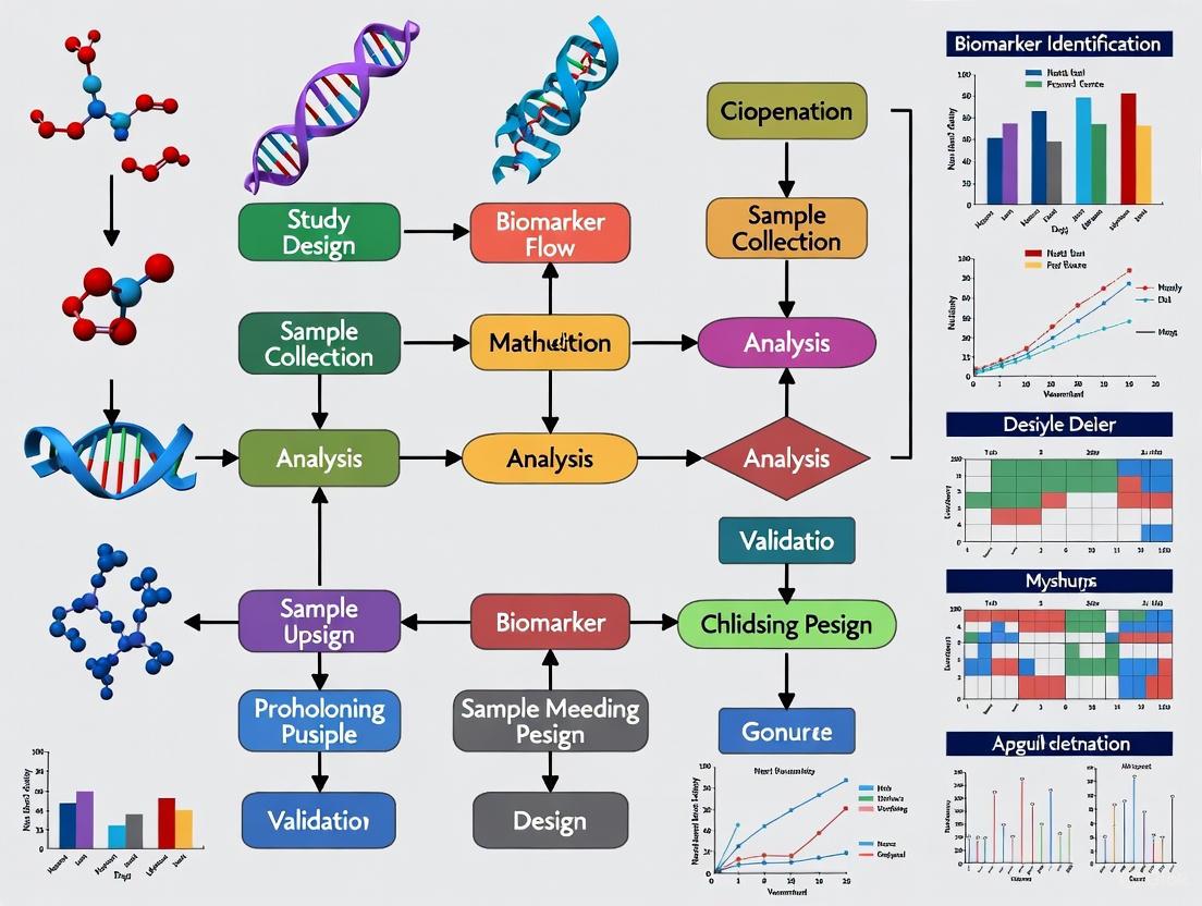
Experimental Workflow and Biomarker Development Pathway
The following diagram illustrates the comprehensive workflow for dietary biomarker development from controlled feeding studies:
Applications in Precision Nutrition and Drug Development
The development of validated dietary biomarkers has far-reaching implications for precision nutrition and pharmaceutical research. In precision nutrition, these biomarkers enable researchers to move beyond one-size-fits-all dietary recommendations toward personalized nutrition approaches that account for individual metabolic variability [3]. The DBDC specifically aims to expand the list of validated biomarkers for foods consumed in the United States diet, which will advance understanding of how diet influences human health and disease risk [3] [1].
In drug development, dietary biomarkers provide crucial tools for assessing dietary exposures in clinical trials, particularly for nutrition-related conditions such as metabolic disorders, cardiovascular disease, and certain cancers [2]. Objective biomarkers help ensure accurate assessment of dietary compliance and can elucidate mechanisms by which diet modifies drug efficacy or toxicity. Furthermore, the three-phase validation approach employed by the DBDC ensures that biomarkers meet rigorous criteria for sensitivity, specificity, and reliability before implementation in research or clinical settings [3] [1].
The integration of dietary biomarkers with other molecular profiling data (genomic, proteomic, metabolomic) creates powerful multidimensional datasets for understanding complex diet-health interactions. As the field advances, these biomarkers will play an increasingly important role in developing targeted nutritional interventions, validating dietary assessment tools, and informing public health policy [3] [1].
Accurate dietary assessment is fundamental to nutrition research, yet traditional self-reported methods, such as food frequency questionnaires and dietary recalls, are plagued by significant measurement error, including substantial underreporting, especially among overweight and obese individuals [2]. Controlled human feeding studies provide a robust alternative by delivering known quantities of specific foods or entire diets, thereby creating a definitive framework for discovering and validating objective biomarkers of food intake (BFIs) [2] [4]. These biomarkers, measured in accessible bio-specimens like blood and urine, offer a pathway to objectively quantify dietary exposure, overcoming the biases inherent in self-report [5] [6]. The central design challenge lies in balancing experimental control with ecological validity. This article details the core methodologies for designing controlled feeding trials, focusing on two principal approaches: the use of standardized menus for all participants and the creation of individualized menus that mimic habitual intake, with a specific focus on their application in dietary biomarker development.
Core Methodologies for Dietary Control
The choice between a standardized or a mimicked habitual diet design is pivotal and depends on the primary research objective. The table below summarizes the key characteristics of each approach.
Table 1: Comparison of Controlled Feeding Study Designs for Biomarker Research
| Feature | Standardized Diet Design | Mimicked Habitual Diet Design |
|---|---|---|
| Primary Objective | To control and isolate the effect of a specific nutrient or food; ideal for mechanistic studies and validating known biomarkers [5]. | To preserve the natural variation in a population's diet; ideal for discovering novel biomarkers across a wide range of foods and for calibration [2] [4]. |
| Diet Composition | Identical menus for all participants, often with a high percentage of energy from a target food (e.g., 80% from ultra-processed foods) [5]. | Unique menus for each participant, designed to approximate their usual food intake as estimated from pre-study dietary records [2]. |
| Key Advantage | High internal validity; reduces inter-individual variance from different food types, preparation, and processing [2]. | Maintains real-world dietary variation, making findings more generalizable to free-living populations [2] [4]. |
| Key Challenge | May be unrepresentative of habitual diets, potentially affecting biomarker metabolism and participant compliance [2]. | Complex and resource-intensive to design and implement; requires extensive dietary interviewing and menu customization [2]. |
| Example Application | NIH clinical trial comparing an 80% ultra-processed food diet to a 0% ultra-processed food diet [5]. | Women's Health Initiative Feeding Study (NPAAS-FS) and the MAIN Study [2] [4]. |
Protocol: Implementing a Mimicked Habitual Diet Design
The following workflow outlines the key steps for implementing a mimicked habitual diet, a complex but powerful design for biomarker discovery.
Figure 1: Workflow for a mimicked habitual diet feeding study.
1. Participant Recruitment and Screening: Recruit participants based on specific inclusion/exclusion criteria. The MAIN Study, for example, excluded individuals with conditions or medications that could alter normal food metabolism, such as diabetes, kidney disease, or cholecystectomy, and required non-vegetarians [4]. Sample size calculations should be based on the expected variation in biomarker levels; the NPAAS-FS targeted 150 participants to have high power (>88%) to detect a biomarker with an R² ≥ 0.5 [2].
2. Baseline Dietary Assessment and Interview: Participants complete a detailed dietary assessment, such as a 4-day food record (4DFR). A critical subsequent step is a standardized, in-depth interview conducted by a study dietitian to assess usual food choices, brands, meal patterns, recipes, and food likes/dislikes not fully captured in the record [2]. This qualitative data is essential for menu personalization.
3. Menu Formulation and Energy Adjustment: Using data from the 4DFR and interview, individualized menus are designed. Energy needs are typically adjusted beyond self-reported intake to prevent non-compliance. In the NPAAS-FS, for 73% of women whose recorded intake was below estimated needs, calories were proportionally increased by an average of 335 ± 220 kcal/day [2]. Software like the Nutrition Data System for Research (NDS-R) and ProNutra is used for nutrient analysis and menu creation [2].
4. Food Provision and Compliance Monitoring: All foods and beverages are provided from a central kitchen. Participants are instructed to consume only the provided foods and to return any uneaten items, allowing for precise calculation of actual intake [2] [4].
Protocol: Implementing a Crossover Trial with Standardized Diets
For investigating the specific effects of a dietary component, a randomized controlled crossover trial is the gold standard.
1. Diet Formulation: Develop two or more tightly controlled diets. A notable example is the NIH study that used a diet comprising 80% of energy from ultra-processed foods versus a diet with 0% ultra-processed foods [5].
2. Randomization and Washout: Participants are randomly assigned to the sequence of diets. Each dietary period is followed by a washout period to allow biomarkers to return to baseline before the next intervention.
3. Controlled Feeding and Biomarker Collection: Participants consume all meals under supervision (e.g., at a clinical center) or as provided take-away meals. Biospecimens are collected at defined time points during each diet phase to capture the metabolic response [5].
The Scientist's Toolkit: Key Reagents and Materials
Successful execution of a controlled feeding study requires meticulous planning and a suite of specialized tools and materials. The following table details essential components of the research toolkit.
Table 2: Research Reagent Solutions for Controlled Feeding Trials
| Tool/Reagent | Function/Description | Example Use in Protocol |
|---|---|---|
| Dietary Analysis Software | Software platforms for nutrient analysis and menu creation. | The NPAAS-FS used NDS-R for analysis and ProNutra for creating menus, recipes, and production sheets [2]. |
| Biospecimen Collection Kits | Standardized kits for the collection, preservation, and transport of biological samples from free-living participants. | The MAIN Study provided participants with kits for home collection of urine samples, demonstrating high compliance and data quality [4]. |
| Doubly Labeled Water (DLW) | A gold-standard recovery biomarker for total energy expenditure (Ein). | Used in the NPAAS-FS as an objective measure to validate energy intake [2]. |
| Urinary Nitrogen | A recovery biomarker for estimating total protein intake. | Measured from 24-hour urine collections in the NPAAS-FS to objectively assess protein consumption [2]. |
| Mass Spectrometry | An analytical platform for metabolomic analysis to identify and quantify metabolite patterns in biospecimens. | Used by NIH researchers to find hundreds of metabolites correlated with ultra-processed food intake and to develop poly-metabolite scores [5]. |
Biomarker Discovery and Validation Workflow
The ultimate goal of many feeding studies is to develop robust biomarkers. The process from biospecimen collection to biomarker validation is multi-staged.
Figure 2: Biomarker discovery and validation pipeline.
Metabolomic Profiling and Machine Learning: As demonstrated in recent NIH research, biospecimens are analyzed using metabolomics to identify metabolites that correlate with dietary intake. Machine learning algorithms can then be employed to identify complex metabolic patterns and calculate a poly-metabolite score—a composite, objective measure of intake that reduces reliance on self-report [5]. This score must subsequently be validated in independent populations with different dietary habits and evaluated for its association with disease outcomes [5].
The strategic design of controlled feeding trials is instrumental in advancing the field of dietary biomarker development. The choice between a standardized menu and a mimicked habitual diet hinges on the research question, with the former offering precision for testing specific hypotheses and the latter providing a realistic variation necessary for discovering and calibrating biomarkers applicable to free-living populations. By adhering to rigorous protocols for diet design, participant management, and biospecimen collection, researchers can generate high-quality data to identify objective biomarkers, ultimately strengthening our understanding of the links between diet and health.
In the field of metabolomics, blood and urine stand as the two most accessible and information-rich biological specimens for discovering and validating dietary biomarkers. Their metabolic profiles provide a functional read-out of the body's physiological state, capturing the complex interplay between diet, metabolism, and health outcomes [7] [8]. For research based on controlled feeding study data, these biofluids are indispensable. Blood metabolomics offers a snapshot of systemic metabolic processes, while urine provides a cumulative record of waste and intermediate products excreted by the kidneys [9]. The non-invasive nature of urine collection and the clinical routine of blood drawing make them ideal for repeated sampling in longitudinal studies, a common feature of feeding trials [10] [9]. The systematic discovery of food intake biomarkers, as championed by initiatives like the Dietary Biomarkers Development Consortium (DBDC), relies on controlled feeding studies coupled with advanced metabolomic profiling of these specimens to identify compounds that are sensitive and specific to dietary exposures [1].
Comparative Analysis of Blood and Urine Specimens
The choice between blood and urine for metabolomic profiling depends on the research question, with each matrix offering distinct advantages and reflecting different biological information. The following table provides a structured comparison for easy reference.
Table 1: Comparative characteristics of blood and urine as specimens for metabolomic profiling.
| Characteristic | Blood (Serum/Plasma) | Urine |
|---|---|---|
| Biological Insight | Snapshot of real-time, systemic metabolism [7] | Cumulative record of metabolic waste and clearance over several hours [9] |
| Invasiveness | Invasive collection | Non-invasive collection [10] [9] |
| Collection Volume | Typically 1-10 mL | Typically 0.25-50 mL [9] |
| Metabolite Stability | Requires rapid processing to prevent glycolysis; highly sensitive to pre-analytical variables [8] | Generally more stable; less sensitive to time-dependent pre-analytical changes post-collection [9] |
| Key Advantages | Captures both endogenous and exogenous metabolites; rich in lipid species; standard for clinical chemistry | High concentration of polar metabolites; ideal for monitoring diurnal variation and long-term exposure [9] |
| Primary Applications | Diagnostic and prognostic biomarker discovery; pathophysiological mechanism investigation [11] [7] | Biomarker discovery for renal and urological diseases; monitoring nutritional interventions and toxic exposures [10] [9] |
Metabolite Classes and Analytical Targets
The metabolome encompassed in blood and urine consists of a diverse range of small molecule metabolites with a molecular mass typically less than 1500 Da [7]. These can be broadly categorized for the purpose of dietary biomarker research.
Table 2: Key classes of metabolites targeted in blood and urine for dietary biomarker discovery.
| Metabolite Class | Representative Members | Primary Biofluid | Role as Dietary Biomarkers |
|---|---|---|---|
| Amino Acids & Derivatives | Branched-chain amino acids, taurine, histidine [11] [7] | Blood, Urine | Markers of protein intake and energy metabolism; disrupted in conditions like colorectal cancer [11] |
| Lipids & Fatty Acids | Glycerophospholipids, sphingolipids, short-chain fatty acids [7] | Blood | Reflect fat intake and energy storage; indicators of cardiovascular health [8] |
| Organic Acids | Citrate, succinate, hippurate [7] | Urine | Products of energy cycles (TCA cycle) and gut microbiota metabolism; sensitive to diet changes [10] |
| Carbohydrates & Derivatives | Glucose, galactose, sugar alcohols | Blood, Urine | Direct markers of sugar and carbohydrate intake [8] |
| Secondary Plant Metabolites | Polyphenols, flavonoids, alkaloids | Urine, Blood | Highly specific biomarkers for intake of fruits, vegetables, and other plant-based foods [1] |
Detailed Experimental Protocols for Specimen Handling
Standardized protocols are critical to ensure the integrity of metabolomic data and the validity of discovered biomarkers. The following sections detail protocols for the collection, processing, and storage of blood and urine specimens in the context of controlled feeding studies.
Blood Collection and Serum/Plasma Processing
This protocol is adapted from methodologies used in large-scale biomarker studies [11].
- Patient Preparation: Participants should fast for 8-16 hours (ideally 12-14 hours) prior to blood collection to minimize the influence of recent dietary intake on the metabolome [11].
- Blood Draw: Collect blood via venipuncture into appropriate collection tubes (e.g., serum separator tubes or EDTA/K2-EDTA tubes for plasma).
- Clotting (for Serum): If serum is required, allow blood to clot at room temperature for 30 minutes.
- Initial Centrifugation: Centrifuge samples at 3000 rpm for 10 minutes at room temperature to separate cells from the liquid fraction.
- Supernatant Transfer & High-Speed Centrifugation: Transfer the supernatant (serum or plasma) to a clean centrifuge tube. Centrifuge again at 14,000 rpm for 10 minutes at 4°C to remove any remaining cellular debris or platelets [11].
- Aliquoting and Storage: Aliquot the clarified serum/plasma into cryovials and immediately freeze at -80°C until analysis. Avoid multiple freeze-thaw cycles.
Urine Collection and Processing
This protocol synthesizes standard practices from clinical metabolomic studies [10] [9].
- Collection: Collect 0.25 to 1 mL of mid-stream urine into a sterile polypropylene tube [9]. Note the fasting status of the participant, if applicable.
- Immediate Storage: Immediately place the specimen into a freezer (≤ -20°C) after collection.
- Centrifugation: Thawed urine samples must be centrifuged at 13,000 rpm for 10 minutes at 4°C to remove any solid debris [10].
- Filtration: Filter the supernatant through a 0.22 μm syringe filter to ensure removal of particulates.
- Long-term Storage: Store the processed urine samples frozen, preferably at -80°C, until ready for shipment and analysis. Ship frozen specimens on dry ice to maintain temperature [9].
Analytical Workflow for Metabolomic Profiling
The journey from a collected biofluid to biomarker discovery involves a multi-step process that integrates laboratory techniques and advanced data analysis. The following diagram illustrates the core workflow.
Diagram 1: Metabolomics biomarker discovery workflow.
Untargeted Metabolomics via Liquid Chromatography-Mass Spectrometry (LC-MS)
The core analytical platform for discovering novel dietary biomarkers is untargeted LC-MS, which allows for the unbiased profiling of thousands of metabolites in a single sample [10] [11] [8].
- Chromatographic Conditions:
- Column: ACQUITY UPLC BEH C18 (e.g., 2.1 mm × 100 mm, 1.7 μm) or HSS T3 column for polar metabolites [10] [11].
- Mobile Phase: Phase A: Water with 0.1% formic acid; Phase B: Acetonitrile with 0.1% formic acid [10] [11].
- Gradient: A typical reverse-phase gradient runs from 1% to 99% organic phase (B) over 10-15 minutes, followed by a re-equilibration step [10].
- Flow Rate: 0.40 mL/min [10].
- Injection Volume: 2-5 μL of processed sample [11].
- Mass Spectrometric Conditions:
- Ionization: Electrospray Ionization (ESI) in both positive and negative ion modes to maximize metabolite coverage [10] [11].
- Mass Analyzer: Quadrupole Time-of-Flight (Q-TOF) or similar high-resolution mass spectrometer for accurate mass measurement [10] [11].
- Mass Range: Full scan from m/z 50 to 1000 [10].
- Capillary Voltage: 2.0 - 3.2 kV [10] [11].
- Source Temperature: 100°C - 110°C; Desolvation Temperature: 200°C - 350°C [10] [11].
- Quality Control: A pooled Quality Control (QC) sample, created by combining a small aliquot of every sample in the study, is analyzed repeatedly throughout the batch to monitor instrument stability and for data normalization [10] [11].
The Scientist's Toolkit: Essential Research Reagents and Materials
Successful metabolomic profiling requires carefully selected reagents and materials to ensure analytical robustness and reproducibility.
Table 3: Essential research reagents and materials for blood and urine metabolomics.
| Item | Function/Application | Example Specifications |
|---|---|---|
| LC-MS Grade Solvents | Used as mobile phases and for sample extraction/reconstitution to minimize background noise and ion suppression. | Acetonitrile, Methanol, Water (all HPLC-MS grade) [10] [11] |
| Acid Additives | Modifies pH of mobile phase to improve chromatographic separation and ionization efficiency in ESI-MS. | Formic Acid (Optima LC/MS grade) [10] [11] |
| Internal Standards | Added to each sample to correct for variability during sample preparation and instrument analysis. | Stable Isotope-Labeled Compound Mixtures (e.g., for targeted analysis) [8] |
| Collection Tubes | For biological specimen collection and initial storage. | Polypropylene Tubes (e.g., Eppendorf Cat #022363204) [9]; EDTA tubes for plasma; serum separator tubes |
| Syringe Filters | Removal of particulate matter from processed urine or protein-precipitated serum samples prior to LC-MS injection. | 0.22 μm, Nylon or PVDF membrane [10] |
| Chromatography Columns | Separation of complex metabolite mixtures based on hydrophobicity before they enter the mass spectrometer. | ACQUITY UPLC BEH C18, 1.7 μm, 2.1x100mm [10] [11] |
| Metabolomics Databases | Annotation and identification of unknown metabolites based on accurate mass, MS/MS fragments, and retention time. | Human Metabolome Database (HMDB), Kyoto Encyclopedia of Genes and Genomes (KEGG) [11] |
Data Analysis and Integration with Feeding Study Data
The raw data generated from LC-MS must be processed to extract meaningful biological information and correlated with dietary intake data from controlled feeding studies.
- Raw Data Conversion: Convert raw mass spectrometer files to an open format (e.g., mzXML) using software like MSConvert [11].
- Peak Processing: Use computational tools like XCMS in R for peak picking, retention time alignment, and feature grouping across all samples. Key parameters include peak width, mass accuracy (ppm), and signal-to-noise threshold [11].
- Multivariate Statistical Analysis: Apply unsupervised (e.g., Principal Component Analysis, PCA) and supervised (e.g., Orthogonal Projections to Latent Structures-Discriminant Analysis, OPLS-DA) methods to identify metabolic features that discriminate between different dietary groups [10] [11].
- Biomarker Identification and Validation: Statistically significant features are identified by querying their accurate mass and MS/MS spectra against metabolomic databases (HMDB, KEGG) [11]. The performance of these candidate biomarkers is then validated in independent sample sets or observational cohorts [1].
- Pathway Analysis: Enrichment analysis tools (e.g., MetaboAnalyst) map the dysregulated metabolites onto biochemical pathways (e.g., primary bile acid biosynthesis, taurine metabolism) to elucidate the biological impact of the dietary intervention [11].
Blood and urine are foundational pillars in the metabolomic assessment of dietary intake. Their complementary nature provides a powerful, multi-faceted view of the metabolic phenotype. The rigorous application of standardized protocols for collection, processing, and analysis, as detailed in these application notes, is paramount for generating high-quality, reproducible data. When integrated with the controlled conditions of feeding studies, metabolomic profiling of these biofluids moves beyond simple correlation to establish causal relationships between diet and metabolic response. This approach is dramatically expanding the list of validated dietary biomarkers, thereby enhancing our ability to objectively assess diet and understand its precise role in health and disease.
Diet is a major modifiable risk factor for chronic diseases, yet accurately assessing dietary intake in free-living populations remains a significant challenge in nutrition research [1]. Current methods, such as food frequency questionnaires and 24-hour recalls, rely on self-reporting and are susceptible to systematic and random measurement errors [1]. To address these limitations, the Dietary Biomarkers Development Consortium (DBDC) was established in 2021 as the first major initiative to systematically discover and validate objective biomarkers for foods commonly consumed in the United States diet [1] [3].
This case study examines the DBDC's Phase 1 approach, which implements controlled feeding trials to identify candidate biomarkers using metabolomic technologies. The consortium's work aims to significantly expand the list of validated dietary biomarkers, thereby enhancing the precision of nutritional science and improving our understanding of diet-health relationships [1] [12].
DBDC Organizational Structure and Governance
The DBDC operates through a coordinated network of research centers and committees overseen by the National Institute of Diabetes and Digestive and Kidney Diseases (NIDDK) and the USDA-National Institute of Food and Agriculture (USDA-NIFA) [1]. The organizational structure ensures rigorous scientific discovery and validation of dietary biomarkers.
Table: DBDC Organizational Structure and Responsibilities
| Component | Institution | Primary Responsibilities |
|---|---|---|
| Study Centers | Harvard University (with Broad Institute), Fred Hutchinson Cancer Center (with University of Washington), University of California Davis (with USDA-ARS) | Conduct controlled feeding trials; collect and process biospecimens; perform metabolomic analyses [1] |
| Data Coordinating Center (DCC) | Duke University | Administrative coordination; data quality control; data analysis for reports; data submission to repositories [1] |
| Steering Committee | Principal investigators from study centers, DCC, NIDDK, and USDA-NIFA | Governing body making strategic scientific and administrative decisions [1] |
| Data Safety Monitoring Board | Independent experts | Regular review of progress, participant safety, data integrity, and scientific rigor [1] |
Three specialized working groups support the consortium's operations: the Dietary Intervention Working Group harmonizes feeding study protocols, the Metabolomics Working Group coordinates analytical methods for biomarker identification, and the Data Analysis/Harmonization Working Group standardizes data collection and analysis plans [1].
Phase 1 Study Designs and Objectives
DBDC Phase 1 employs controlled feeding trials to identify candidate biomarkers and characterize their pharmacokinetic parameters. The three study centers implement complementary research protocols focused on different food groups [1] [13].
Table: DBDC Phase 1 Study Characteristics
| Research Center | Primary Food Focus | Study Status | Key Objectives |
|---|---|---|---|
| UC Davis Dietary Biomarker Development Center | Fruits and vegetables [13] [14] | Recruiting [13] | Identify biomarkers linked to specific fruits and vegetables; determine dose and time responses of metabolites [15] |
| Dietary Biomarker Intervention Core (Harvard) | Proteins (chicken, beef, salmon, soybeans), carbohydrates (whole wheat, potatoes, corn, oats), and dairy (yogurt, cheese) [13] [14] | Recruiting [13] | Conduct tightly controlled pharmacokinetic and dose-response feeding studies across range of food items [13] |
| Seattle Dietary Biomarker Development Center (Fred Hutch) | USDA MyPlate foods, food groups, and dietary patterns [13] [16] | Recruiting [13] | Discover biomarkers of MyPlate food groups/subgroups; determine half-lives and dynamic range [17] |
The overarching goal of Phase 1 is to identify sensitive and specific candidate biomarkers by administering test foods in prespecified amounts to healthy participants and conducting metabolomic profiling of blood and urine specimens collected during feeding trials [1]. Data from these studies will characterize the pharmacokinetic parameters of candidate biomarkers associated with specific foods [1].
Experimental Protocols and Methodologies
Participant Recruitment and Controlled Feeding
Each DBDC center recruits healthy adult participants for controlled feeding studies [13]. Prior to intervention, habitual diet is assessed using food frequency questionnaires (FFQs) and recent intake is evaluated through automated 24-hour dietary recalls (ASA-24) [15]. The feeding studies employ standardized protocols:
- Test Meals: Participants consume test foods in prespecified amounts following randomized controlled dietary intervention designs [15]. The UC Davis center, for example, administers different servings of fruit and vegetable mixtures in an inverse dosing gradient (e.g., 1 fruit/3 vegetables, 2 fruit/2 vegetables, 3 fruit/1 vegetables) within a standard mixed meal setting [15].
- Dietary Control: Participants are provided with standardized meals and snacks low in the target food groups to prevent interference with biomarker detection [15].
- Washout Periods: Multiple dosing interventions are conducted with at least 48-hour washout periods between test sessions [15].
Biospecimen Collection and Processing
Comprehensive biospecimen collection is critical for metabolomic analysis in Phase 1 studies:
- Blood Collection: Fasting blood samples are collected initially, followed by postprandial samples at 1, 2, 4, 6, and 8 hours after test meal consumption. A final fasting sample is collected at 24 hours [15].
- Urine Collection: Urine is pooled sequentially between 0-2, 2-4, 4-6, and 6-8 hours, with a final collection from 8-24 hours [15].
- Sample Processing: All biospecimens are processed, tracked, and stored according to standardized protocols across centers to maintain sample integrity [1] [17].
Diagram Title: DBDC Phase 1 Experimental Workflow
Metabolomic Profiling and Biomarker Discovery
Phase 1 utilizes advanced metabolomic technologies to identify candidate biomarkers:
- Analytical Platforms: Liquid chromatography-mass spectrometry (LC-MS) and hydrophilic-interaction liquid chromatography (HILIC) are employed for comprehensive metabolite profiling [1]. Both untargeted and targeted approaches are used to discover novel biomarkers and quantify known compounds [15] [17].
- Metabolite Identification: Unknown metabolites are characterized using high-resolution MS/MS with ramped collision energies and SWATH-based LC-TripleTOF MS to ensure accurate identification with associated retention times and precise masses [15].
- Quality Assurance: Extensive QA/QC strategies are implemented to ensure analytical precision and stability, including analysis of blinded duplicate samples [15] [17].
Data Analysis and Statistical Approaches
The DBDC employs sophisticated statistical methods to identify and validate dietary biomarkers:
- Kinetic Modeling: Data analysis cores characterize the appearance and clearance kinetics of metabolites in blood and urine to determine optimal sampling times and stratify markers for acute or habitual intake [15].
- Generalized Linear Models: Multiple GLM approaches (Gaussian, log-link Gaussian, log-normal, etc.) are constructed, adjusting for subject metadata and using participants as random effects to evaluate intervention-associated changes in biomarkers [15].
- Bayesian Methods: Effect sizes are estimated using Bayesian regression with credible intervals >95% to account for interindividual variability stemming from genetics, lifestyle, gut microbiome, and ADME profiles [15].
- Multiple Comparison Correction: The false discovery rate is controlled using the Benjamini-Hochberg method to ensure statistical rigor in biomarker identification [1].
The Scientist's Toolkit: Research Reagent Solutions
Table: Essential Research Materials and Analytical Tools for Dietary Biomarker Studies
| Item/Category | Function/Application | Examples/Specifications |
|---|---|---|
| Liquid Chromatography-Mass Spectrometry (LC-MS) | Primary platform for metabolomic profiling; separates and detects small molecules in biospecimens [1] | Ultra-HPLC (UHPLC) systems coupled to high-resolution mass spectrometers [1] |
| Hydrophilic-Interaction Liquid Chromatography (HILIC) | Complementary separation mechanism for polar metabolites; enhances coverage of metabolome [1] | HILIC columns with MS-compatible mobile phases [1] |
| Chemical Libraries & Standards | Metabolite identification; quantification; method development and validation [1] | Commercially available metabolite standards; in-house generated spectral libraries [15] |
| Stable Isotope-Labeled Compounds | Tracking metabolite fate; distinguishing dietary compounds from endogenous metabolites [15] | ¹³C, ¹⁵N-labeled analogs of suspected biomarkers |
| Quality Control Materials | Monitoring analytical performance; ensuring data quality across batches and sites [15] [17] | Pooled reference samples; blinded duplicates; standard reference materials [17] |
Significance and Future Directions
The DBDC Phase 1 approach represents a transformative advancement in nutritional science by applying rigorous metabolomic technologies to the challenge of dietary assessment. The discovery and validation of objective food biomarkers will address critical limitations of self-reported dietary data and enhance the precision of nutrition research [1] [14].
Following Phase 1, the DBDC will progress to Phase 2, where candidate biomarkers will be evaluated for their ability to identify individuals consuming biomarker-associated foods using controlled feeding studies of various dietary patterns [1]. Phase 3 will validate the most promising biomarkers in independent observational settings to predict recent and habitual consumption of specific test foods [1].
All data generated throughout the DBDC study phases will be archived in publicly accessible databases, including the NIDDK Central Repository and Metabolomics Workbench, serving as a valuable resource for the broader research community [1]. This systematic approach promises to significantly expand the repertoire of validated dietary biomarkers, ultimately advancing our understanding of how diet influences human health and disease.
Establishing Pharmacokinetic Parameters and Dose-Response Relationships
Within the framework of biomarker development from controlled feeding studies, the precise establishment of pharmacokinetic (PK) parameters and dose-response relationships is fundamental. These quantitative assessments form the critical link between dietary exposure and biological effect, allowing researchers to move from simple observational associations to a mechanistic understanding of how foods and nutrients influence health. PK parameters describe the body's processing of a compound—its absorption, distribution, metabolism, and excretion (ADME)—while dose-response modeling quantifies the relationship between the exposure level and the magnitude of a biological response [18]. In the specific context of the Dietary Biomarkers Development Consortium (DBDC), the goal is to discover and validate objective biomarkers for foods consumed in the U.S. diet, a process that relies heavily on controlled feeding trials and subsequent metabolomic profiling to identify candidate compounds that reliably reflect intake [3]. This document outlines detailed protocols and applications for determining these essential parameters to advance the field of precision nutrition.
Core Concepts and Definitions
Fundamental Pharmacokinetic Parameters
Pharmacokinetics describes "what the body does to a drug"—or, in a nutritional context, a bioactive food component. The key parameters are summarized in the table below. These parameters are typically assessed by monitoring the concentration-time profile of a compound or its metabolites in accessible biological fluids like plasma or urine [19].
Table 1: Key Pharmacokinetic Parameters and Their Definitions
| Parameter | Symbol | Definition | Significance |
|---|---|---|---|
| Area Under the Curve | AUC | Total exposure to a compound over time | Surrogate for total drug exposure; used to calculate bioavailability [19] |
| Maximum Concentration | C~max~ | Peak plasma concentration after administration | Indicates the intensity of exposure [19] |
| Time to C~max~ | T~max~ | Time taken to reach peak concentration | Reflects the rate of absorption [19] |
| Elimination Half-Life | t~1/2~ | Time for plasma concentration to reduce by 50% | Determines dosing frequency and time to steady-state [20] [19] |
| Clearance | CL | Volume of plasma cleared of the compound per unit time | Represents the body's efficiency in eliminating the compound [19] |
| Volume of Distribution | V~d~ | Apparent volume in which a compound distributes | Indicates extent of distribution outside the plasma compartment [19] |
| Bioavailability | F | Fraction of administered dose that reaches systemic circulation | Critical for evaluating efficacy of extravascular routes (e.g., oral) [20] [19] |
Principles of Dose-Response Modeling
The dose-response relationship, a cornerstone of toxicology and pharmacology, describes the magnitude of a biological response as a function of exposure level [21]. Dose-response modeling quantitatively assesses this relationship to identify which exposure doses are safe, hazardous, or beneficial [22]. These relationships are typically visualized through dose-response curves, which are often sigmoidal in shape when the dose is plotted on a logarithmic scale [21].
Key metrics derived from these models include:
- Potency: Often represented by the EC~50~ (half maximal effective concentration) or ED~50~ (half maximal effective dose), which is the dose required to produce 50% of the maximum response [21].
- Efficacy: Represented by E~max~, the maximum possible effect a compound can elicit [21].
- Benchmark Dose (BMD): The dose that produces a predetermined, measurable change in response rate (Benchmark Response, or BMR), often a 5% or 10% change from background. The BMDL is the lower confidence bound of the BMD and is often used as a Point of Departure (POD) for risk assessment [22] [23].
Experimental Protocols
Protocol 1: Determining PK Parameters from a Controlled Feeding Study
This protocol outlines the methodology for characterizing the pharmacokinetics of a dietary biomarker following a controlled dose, aligned with the controlled feeding trials described by the DBDC [3].
1. Study Design and Dosing:
- Subjects: Recruit healthy participants. The study protocol must be approved by an Institutional Review Board (IRB) and/or an Animal Care and Use Committee (IACUC) for preclinical studies [18].
- Administration: Administer a precise, pre-specified amount of the test food or nutrient. The route should mimic typical consumption (e.g., oral). An intravenous dose of a purified compound may be co-administered in a separate phase to determine absolute bioavailability [18].
- Controls: Implement appropriate control diets to account for background metabolic interference.
2. Sample Collection:
- Collect serial blood samples (e.g., plasma, serum) at predetermined time points: pre-dose, and at multiple time points post-dose (e.g., 0.5, 1, 2, 4, 8, 12, 24 hours) to fully characterize the absorption and elimination phases [18].
- Collect urine over timed intervals (e.g., 0-4h, 4-8h, 8-12h, 12-24h) to determine renal excretion.
- Immediately process samples (e.g., centrifugation for plasma) and store at -80°C until analysis.
3. Bioanalytical Analysis:
- Use targeted or untargeted metabolomic approaches, such as Liquid Chromatography-Mass Spectrometry (LC-MS), to quantify the candidate biomarker and its potential metabolites in the biological samples [3].
- Ensure method validation for accuracy, precision, and sensitivity.
4. Data Analysis and Parameter Calculation:
- Plot the plasma concentration-time curve for each subject.
- Use non-compartmental analysis (NCA) to calculate PK parameters [19]:
- AUC: Calculate using the trapezoidal rule.
- C~max~ and T~max~: Observed directly from the data.
- Elimination Rate Constant (K): Determine by performing linear regression on the log-linear portion of the concentration-time curve [24]. The half-life is then calculated as ( t{1/2} = 0.693 / K ) [24].
- Clearance (CL): For intravenous dosing, ( CL = Dose / AUC ). For oral dosing, ( CL = F \cdot Dose / AUC ), where F is bioavailability.
- Volume of Distribution (V~d~): ( Vd = CL / K ) [24].
The following diagram illustrates the workflow for this protocol:
Protocol 2: Establishing a Dose-Response Relationship
This protocol describes the steps for modeling the relationship between the dose of a nutrient and a measurable health outcome, which is central to risk-benefit assessment (RBA) [25].
1. Experimental Design:
- Dose Groups: Assign subjects or animals to multiple groups receiving different doses of the nutrient or food of interest, including a control (zero-dose) group. A wide range of doses is preferable.
- Endpoint Measurement: Define and measure a relevant quantitative endpoint. This could be a continuous outcome (e.g., blood pressure, biomarker concentration) or a quantal outcome (e.g., incidence of tumors) [22] [23].
2. Data Plotting and Model Selection:
- Plot the raw data with dose on the x-axis and response on the y-axis.
- Test several mathematical models to find the best fit for the data. Common models include:
- Hill Equation: ( E = E{0} + \frac{[A]^n \times E{max}}{[A]^n + EC_{50}^n} ) , where E is the effect, E₀ is the baseline effect, [A] is the dose, E~max~ is the maximum effect, EC~50~ is the half-maximally effective dose, and n is the Hill coefficient that determines steepness [21] [26].
- Weibull Model
- Logistic Model
3. Model Fitting and Evaluation:
- Fit the candidate models to the data using nonlinear regression techniques.
- Evaluate the goodness-of-fit using statistical criteria such as Akaike's Information Criterion (AIC) or the Bayesian Information Criterion (BIC). Visually inspect the curve fit.
4. Derivation of Benchmark Doses (BMD):
- Define a Benchmark Response (BMR), which is a predetermined change in response (e.g., 10% increase over background).
- Using the best-fitting model, calculate the BMD—the dose corresponding to the BMR.
- Calculate the BMDL, the lower confidence bound of the BMD (e.g., the 95% lower confidence limit) [22] [23].
Table 2: Common Dose-Response Model Functions
| Model Name | Function | Typical Application |
|---|---|---|
| Hill Equation | ( E = E{0} + \frac{[A]^n \times E{max}}{[A]^n + EC_{50}^n} ) | Standard model for efficacy and potency; widely used in pharmacology [21] [26] |
| Linear Model | ( E = E_{0} + k \cdot [A] ) | Simple linear relationships; often used for low-dose extrapolation |
| Weibull Model | ( E = E{0} + E{max} (1 - e^{-([A]/k)^m}) ) | Flexible model for toxicological data with a threshold-like shape |
The Scientist's Toolkit: Research Reagent Solutions
Table 3: Essential Reagents and Materials for PK and Dose-Response Studies
| Item | Function/Application |
|---|---|
| Liquid Chromatography-Mass Spectrometry (LC-MS/MS) | High-sensitivity quantification and identification of biomarkers and metabolites in complex biological matrices like plasma and urine [3]. |
| Stable Isotope-Labeled Standards | Internal standards for mass spectrometry that correct for matrix effects and recovery losses, ensuring analytical accuracy and precision. |
| Biomarker Discovery Panels | Multiplexed assays for broad-spectrum metabolomic or proteomic profiling to identify novel candidate biomarkers in controlled feeding studies [3]. |
| Pharmacokinetic Modeling Software | Software platforms (e.g., NONMEM, Phoenix WinNonlin) for performing non-compartmental and compartmental analysis to calculate PK parameters [26]. |
| Benchmark Dose Software (BMDS) | US EPA-developed software for conducting dose-response modeling and deriving benchmark doses (BMD/BMDL) for risk assessment [23]. |
| Controlled Diet Formulations | Precisely formulated diets for feeding studies, ensuring consistent and reproducible nutrient exposure for all participants or animals [3]. |
Integrated Workflow: From Feeding Study to Biomarker Validation
The integration of PK and dose-response analysis is critical for biomarker development. The DBDC outlines a three-phase approach that encapsulates this integration [3]:
- Phase 1: Discovery: Controlled feeding trials with test foods are conducted, and biospecimens are analyzed using metabolomics to identify candidate biomarker compounds and characterize their pharmacokinetic parameters.
- Phase 2: Evaluation: The ability of candidate biomarkers to classify consumers vs. non-consumers is tested using controlled feeding studies of various dietary patterns.
- Phase 3: Validation: The validity of candidate biomarkers to predict habitual intake is evaluated in independent observational cohorts.
The relationship between PK/PD modeling and the broader goal of biomarker development can be visualized as follows, showing how different modeling approaches feed into the validation pipeline:
Application in Nutritional Science: A Case Study on Fibre and Calcium
Quantitative dose-response relationships are increasingly used in food risk-benefit assessment (RBA). A recent synthesis of meta-analyses revealed specific, quantifiable relationships between nutrient intake and health outcomes [25]:
- Dietary Fibre: A dose-response relationship shows a protective effect against colorectal cancer, with cereal fibre being the most beneficial source. The relationship can be quantified as a specific percentage reduction in risk per gram of fibre consumed.
- Calcium: Inverse associations were found with several cancers. However, the relationship is complex, as high dairy intake (a primary calcium source) may be associated with an increased risk of prostate cancer, highlighting the importance of considering the nutrient source.
- Zinc: Exhibits a potential U-shaped relationship with colorectal cancer risk, indicating that both deficiency and excessive intake may be harmful.
These findings underscore the power of dose-response modeling to move beyond qualitative advice ("eat more fibre") to quantitative, evidence-based dietary recommendations.
Advanced Techniques and Analytical Approaches for Biomarker Identification
The pursuit of objective biomarkers for dietary intake represents a significant frontier in nutritional epidemiology and precision health. Diet is a complex exposure that profoundly affects health across the lifespan, yet accurately assessing dietary intake through self-reported methods remains challenging. Objective biomarkers that can reliably reflect intake of specific nutrients, foods, and dietary patterns are therefore critically needed to strengthen research on diet-health relationships [3]. Within this context, liquid chromatography-mass spectrometry (LC-MS) coupled with hydrophilic interaction liquid chromatography (HILIC) has emerged as a powerful analytical platform for discovering and validating dietary biomarkers. These technologies enable comprehensive profiling of the complex metabolome present in biological samples, capturing the subtle metabolic changes induced by specific dietary components.
The Dietary Biomarkers Development Consortium (DBDC) exemplifies the systematic approach required for this endeavor, implementing a 3-phase framework for biomarker discovery and validation that spans controlled feeding trials to independent observational studies [3]. Success in this domain requires not only advanced instrumentation but also rigorous experimental protocols, optimized chromatographic separations, and sophisticated data analysis pipelines. This application note provides detailed methodologies for leveraging LC-MS and HILIC platforms to advance compound identification in metabolomics studies, with particular emphasis on applications within controlled feeding studies for biomarker development.
Analytical Workflow for Metabolite Identification
The complete workflow for metabolite identification in biomarker development studies encompasses multiple stages from sample preparation through data interpretation. The following diagram illustrates this integrated process:
Figure 1: Integrated workflow for metabolite identification in biomarker development studies
Materials and Reagents
Research Reagent Solutions
Table 1: Essential research reagents and materials for LC-MS/HILIC metabolomics
| Reagent/Material | Specifications | Function in Workflow |
|---|---|---|
| Mobile Phase A | 10 mM ammonium formate/acetate in water, pH 3.0 ( Ultra LC-MS grade) | Aqueous component for HILIC separation; volatile buffer enhances ionization |
| Mobile Phase B | Acetonitrile with 0.1% formic acid (Ultra LC-MS grade) | Organic component for HILIC separation; maintains compound retention |
| Protein Precipitation Solvent | 80% methanol in water (LC-MS grade) | Deproteinization of plasma/serum samples; metabolite extraction |
| Reference Standards | >95% purity, 1.0 mg/mL in 80% methanol (MetaSci, Sigma-Aldrich) | Compound identification and retention time calibration |
| HILIC Column | Sulfobetaine-based Atlantis Premier BEH Z-HILIC (2.1 × 100 mm, 1.7 µm) | Separation of polar metabolites; minimal analyte adsorption |
| Quality Control | Pooled plasma sample from study cohort | Monitoring instrument performance; data normalization |
Instrumentation Specifications
Modern metabolomics relies on complementary instrumental configurations to balance comprehensive coverage with sensitive quantification. The EMBL-MCF 2.0 method utilizes two complementary platforms [27]:
- Untargeted Discovery Platform: Biocompatible Vanquish Horizon UHPLC system (MP35N-based) coupled to Orbitrap Exploris 240 mass spectrometer
- Targeted Validation Platform: Exion LC AD system coupled to QTRAP 6500+ mass spectrometer
The utilization of low-adsorption LC hardware (MP35N, PEEK, titanium) is critical for minimizing loss of metabolites containing common functional groups such as phosphates and carboxylates that exhibit non-specific adsorption to metal and stainless-steel surfaces [27].
Experimental Protocols
Sample Preparation Protocol
Proper sample preparation is fundamental to achieving reproducible results in metabolomics. The following protocol is optimized for plasma/serum samples from controlled feeding studies:
- Thawing: Slowly thaw plasma samples on ice for 30-60 minutes.
- Aliquoting: Transfer 100 µL of plasma to a low-adsorption microcentrifuge tube.
- Protein Precipitation: Add 400 µL of pre-chilled 80% methanol (-20°C) to the plasma.
- Vortexing and Incubation: Vortex thoroughly for 30 seconds, then incubate at -20°C for 20 minutes.
- Centrifugation: Centrifuge at 14,000 × g for 15 minutes at 4°C.
- Collection: Carefully transfer 400 µL of supernatant to a new low-adsorption vial without disturbing the protein pellet.
- Storage: Store extracts at -80°C until LC-MS analysis (typically within 48 hours).
- Quality Control: Prepare a pooled QC sample by combining 50 µL aliquots from each processed sample [27].
HILIC Chromatography Method
HILIC separation is particularly valuable for retaining highly polar metabolites that elute near the void volume in reversed-phase chromatography. The following method provides robust retention and separation of polar compounds:
Table 2: HILIC chromatographic conditions for polar metabolite separation
| Parameter | Specification | Notes |
|---|---|---|
| Column | Atlantis Premier BEH Z-HILIC (2.1 × 100 mm, 1.7 µm) | Sulfobetaine-based chemistry; excellent for acids and bases |
| Column Temperature | 40°C | Enhanced reproducibility and peak shape |
| Flow Rate | 0.4 mL/min | Optimal for MS sensitivity and separation |
| Injection Volume | 3 µL | Compromise between sensitivity and matrix effects |
| Gradient Timetable | Time (min) | % Mobile Phase B (ACN) |
| 0.0 | 85% | |
| 1.0 | 85% | |
| 10.0 | 20% | |
| 11.0 | 20% | |
| 11.5 | 85% | |
| 15.0 | 85% | |
| Autosampler Temperature | 4°C | Maintains sample integrity |
This method employs a decreasing organic gradient to elute compounds based on increasing hydrophilicity, with the initial high organic content (85% acetonitrile) ensuring proper retention on the HILIC stationary phase [27].
Mass Spectrometry Acquisition Parameters
Data acquisition in biomarker discovery studies typically employs both high-resolution full-scan and targeted MS/MS modes:
Table 3: Mass spectrometry parameters for untargeted and targeted analysis
| Parameter | Untargeted (Orbitrap) | Targeted (QTRAP) |
|---|---|---|
| Ionization Mode | Electrospray ionization (ESI) positive/negative switching | ESI positive or negative mode |
| Spray Voltage | ±3.5 kV | ±4.5 kV |
| Sheath Gas | 50 arb | 50 arb |
| Aux Gas | 10 arb | 10 arb |
| Capillary Temperature | 320°C | 500°C |
| MS1 Resolution | 120,000 @ m/z 200 | Unit resolution (Q1) |
| Scan Range | m/z 70-1050 | MRM transitions |
| MS2 Acquisition | Data-dependent acquisition (top 10) | Optimized collision energies |
| Collision Energy | Stepped (20, 35, 50 eV) | Compound-specific |
| Chromatographic Peak Width | ≥ 4 scans/peak | ≥ 12 data points/peak |
The dual-platform approach enables comprehensive metabolite profiling in discovery phase (Orbitrap) followed by sensitive and quantitative validation of candidate biomarkers (QTRAP) [27].
Data Analysis and Compound Identification
Statistical Approaches for Biomarker Discovery
The analysis of metabolomics data requires careful consideration of statistical methods, particularly as the number of metabolites increases. Comparative studies have demonstrated that:
- With small sample sizes (N < 200) and targeted metabolomics (∼200 metabolites), traditional univariate methods with false discovery rate (FDR) correction perform adequately.
- With larger sample sizes (N > 1000) and nontargeted metabolomics (∼2000 metabolites), sparse multivariate methods such as Sparse Partial Least Squares (SPLS) and LASSO regression demonstrate superior performance with higher positive predictive value and fewer false positives [28].
The improved performance of multivariate methods in high-dimensional data stems from their ability to model the complex correlation structure between metabolites, reducing spurious associations that may arise due to intercorrelation with true positive metabolites [28].
Advanced Annotation with Network Analysis
Global network optimization approaches have revolutionized compound identification in untargeted metabolomics. The NetID algorithm exemplifies this strategy by:
- Connecting ion peaks based on mass differences reflecting adduct formation, fragmentation, isotopes, or feasible biochemical transformations
- Applying integer linear programming to achieve global optimization of network annotations
- Differentiating biochemical connections from mass spectrometry phenomena based on chromatographic co-elution
- Scoring candidate annotations based on mass accuracy, retention time alignment, and MS/MS spectral similarity [29]
This approach generates a single consistent network linking most observed ion peaks, substantially improving annotation coverage and accuracy compared to individual peak annotation strategies. The network-based methodology is particularly valuable for identifying previously unrecognized metabolites, such as thiamine derivatives and N-glucosyl-taurine, through their biochemical relationships to known metabolites [29].
The following diagram illustrates the network-based annotation process:
Figure 2: Network-based annotation workflow for metabolite identification
Application in Biomarker Development
Integration with Controlled Feeding Studies
The DBDC has established a systematic 3-phase framework for biomarker development that integrates controlled feeding studies with advanced metabolomics:
- Phase 1 - Discovery: Controlled feeding of test foods in prespecified amounts to healthy participants followed by metabolomic profiling to identify candidate compounds and characterize their pharmacokinetic parameters [3].
- Phase 2 - Evaluation: Assessment of candidate biomarkers' ability to identify individuals consuming specific foods using controlled feeding studies of various dietary patterns [3].
- Phase 3 - Validation: Evaluation of candidate biomarkers' predictive validity for recent and habitual consumption in independent observational settings [3].
This phased approach ensures that biomarkers progress through increasingly rigorous testing before implementation in epidemiological studies.
Biological Interpretation Tools
Specialized computational tools have been developed to facilitate biological interpretation of metabolomics data in specific domains. The Immunometabolic Atlas (IMA) exemplifies such tools by:
- Inferring associations between metabolites and immune processes through protein-metabolite network analysis
- Leveraging Gene Ontology annotations and protein-metabolite interaction databases
- Enabling inheritance of immune process associations by metabolites based on their protein interactions [30]
Similar approaches can be adapted for nutritional metabolomics by creating networks that connect metabolites to specific dietary exposures through biochemical pathways.
The integration of LC-MS/HILIC platforms with robust experimental protocols and advanced computational methods provides a powerful framework for compound identification in biomarker development research. The methodologies detailed in this application note—from sample preparation through network-based annotation—enable researchers to confidently identify metabolites associated with specific dietary exposures in controlled feeding studies. As the field progresses toward standardized biomarker development pipelines, these protocols offer a foundation for generating reproducible, high-quality metabolomics data that can advance precision nutrition and enhance our understanding of diet-health relationships.
Machine Learning and AI Algorithms for Pattern Recognition in Complex Datasets
The discovery and validation of dietary biomarkers represent a significant challenge in nutritional science and precision medicine. Objective biomarkers are crucial for accurately assessing associations between diet and health outcomes, as traditional self-reported dietary measures are often limited by their reliability and validity [3]. Machine learning (ML) and artificial intelligence (AI) algorithms have emerged as powerful tools for identifying subtle patterns in complex biological datasets generated from controlled feeding studies. These algorithms can analyze high-dimensional data from metabolomics, metagenomics, and other profiling technologies to identify compounds and biological features that serve as sensitive and specific biomarkers of dietary exposures [3] [31].
The application of ML in biomarker development represents a paradigm shift from traditional statistical approaches. ML algorithms excel at identifying complex, non-linear relationships within high-dimensional data that might elude conventional analysis methods. For researchers and drug development professionals, this capability is particularly valuable for understanding how dietary components influence physiological processes and disease risk, ultimately supporting the development of targeted nutritional interventions and therapies.
Key Machine Learning Algorithms for Pattern Recognition
Algorithm Classification and Applications
Machine learning algorithms can be categorized based on their learning approach, each with distinct strengths for biomarker discovery applications.
Supervised learning algorithms learn from labeled training data, where both input data and corresponding output labels are provided [32]. This approach is analogous to a teacher providing examples with answers, enabling the algorithm to later make predictions on new, unlabeled data [32]. In the context of biomarker development, supervised learning is particularly valuable for classification tasks, such as determining whether specific dietary exposures have occurred based on biological samples.
Unsupervised learning algorithms identify inherent patterns, structures, or groupings within data without pre-existing labels [32]. This approach is likened to organizing a messy closet without instructions, making it valuable for discovering previously unknown subtypes or patterns in biological data that may represent novel biomarker signatures [32].
Ensemble methods combine multiple models to improve predictive performance and robustness. These methods are particularly effective for complex biomarker discovery tasks where multiple weak predictors can be combined to form a stronger overall model.
Table 1: Machine Learning Algorithms for Biomarker Development
| Algorithm | Type | Primary Use in Biomarker Research | Key Advantages |
|---|---|---|---|
| Random Forest | Supervised | Classification of dietary intake based on metagenomic features [33] [31] | Handles high-dimensional data well; reduces overfitting through ensemble approach [33] |
| Logistic Regression | Supervised | Binary classification of dietary exposure [33] [32] | Provides probability estimates; efficient with smaller datasets [33] |
| K-nearest neighbor (KNN) | Supervised | Pattern recognition in metabolic profiles [33] | Simple implementation; effective for multi-class problems [33] |
| Support Vector Machine (SVM) | Supervised | Classification in high-dimensional biomarker data [33] | Effective with small sample sizes; reliable performance [33] |
| K-means | Unsupervised | Clustering of similar metabolic response patterns [33] | Identifies natural groupings in data without pre-defined labels [33] |
| Gradient Boosting | Supervised | Creating strong predictive models from weak learners [33] | High predictive accuracy; handles complex patterns well [33] |
| Naive Bayes | Supervised | Probabilistic classification of dietary patterns [33] | Works well with high-dimensional data; computationally efficient [33] |
Algorithm Selection Considerations
Selecting appropriate machine learning algorithms for biomarker development requires careful consideration of multiple factors. Dataset dimensionality is a primary concern, as high-dimensional omics data may benefit from algorithms like random forest that naturally handle many features [33] [31]. Sample size availability also influences algorithm choice, with support vector machines performing reliably even with smaller sample sizes [33]. The specific research question further guides selection, with classification problems requiring different approaches than clustering or pattern discovery tasks. For dietary biomarker development, random forest has demonstrated particular utility, achieving 80-87% classification accuracy for specific food intake in controlled feeding studies [31].
Experimental Protocols for Biomarker Discovery
Controlled Feeding Study Design
The Dietary Biomarkers Development Consortium (DBDC) has established a rigorous 3-phase approach for biomarker discovery and validation that integrates machine learning at multiple stages [3].
Phase 1: Candidate Biomarker Identification
- Participant Administration: Healthy participants receive test foods in prespecified amounts under controlled conditions [3]
- Sample Collection: Blood and urine specimens are collected at predetermined timepoints following dietary administration [3]
- Metabolomic Profiling: Advanced analytical techniques including liquid chromatography-mass spectrometry (LC-MS) are employed to generate comprehensive metabolic profiles [3]
- Pharmacokinetic Characterization: Data from feeding trials characterize pharmacokinetic parameters of candidate compounds associated with specific foods [3]
Phase 2: Biomarker Evaluation
- Controlled feeding studies utilizing various dietary patterns assess the ability of candidate biomarkers to identify individuals consuming biomarker-associated foods [3]
- Machine learning models are trained to classify dietary exposure based on candidate biomarker profiles
- Algorithm performance is evaluated using cross-validation techniques to ensure robustness
Phase 3: Biomarker Validation
- Candidate biomarkers are evaluated in independent observational settings [3]
- Models predict recent and habitual consumption of specific test foods [3]
- Validation against traditional dietary assessment methods establishes real-world utility [3]
Metagenomic Biomarker Discovery Protocol
Recent research has demonstrated the utility of fecal metagenomics for developing objective biomarkers of food intake. The following protocol outlines key experimental steps:
Sample Processing and DNA Sequencing
- Fecal samples are collected at pre- and post-intervention timepoints in controlled feeding studies [31]
- DNA extraction is performed using standardized protocols to ensure sample integrity
- Shotgun genomic sequencing generates comprehensive metagenomic data [31]
Data Preprocessing and Functional Annotation
- Raw sequencing data undergoes quality control and preprocessing to remove artifacts and ensure data quality [31]
- Sequences are aligned using specialized tools such as Double Index AlignMent Of Next-generation sequencing Data (v2.0.11.149) [31]
- Functional annotation is performed using platforms like MEtaGenome ANalyzer (MEGAN, v6.12.2) to identify genes and metabolic pathways [31]
Differential Abundance Analysis
- Normalized count data is transformed using log fold change ratios between pre- and post-intervention samples [31]
- Differential abundance analysis identifies Kyoto Encyclopedia of Genes and Genomes (KEGG) Orthology categories that significantly change with specific food intake [31]
- Statistical thresholds (e.g., q < 0.20) control for false discovery in high-dimensional data [31]
Machine Learning Model Development
- Differentially abundant features are used as input for random forest classification models [31]
- Both single-food and multi-food models are developed to test classification accuracy [31]
- Model performance is evaluated using appropriate validation techniques to ensure generalizability
Table 2: Performance of Metagenomic Biomarker Classification
| Food Item | Number of Significant KEGG Orthologies | Classification Accuracy | Model Type |
|---|---|---|---|
| Almond | 54 | 80% | Random Forest [31] |
| Broccoli | 2,474 | 87% | Random Forest [31] |
| Walnut | 732 | 86% | Random Forest [31] |
| Mixed Food Model | Combined Features | 81% | Random Forest [31] |
Data Visualization and Workflow
Biomarker Discovery Workflow - This diagram illustrates the comprehensive workflow from controlled feeding studies to biomarker validation, highlighting the integration of machine learning at key analytical stages.
Random Forest Classification - This visualization shows the ensemble approach of random forest algorithms used to classify food intake based on metagenomic features, with multiple decision trees contributing to a final classification through majority voting.
The Scientist's Toolkit: Research Reagent Solutions
Table 3: Essential Research Reagents and Platforms for ML-Driven Biomarker Discovery
| Reagent/Platform | Function | Application in Biomarker Research |
|---|---|---|
| Liquid Chromatography-Mass Spectrometry (LC-MS) | Separation and detection of metabolic compounds | Profiling of blood and urine specimens for candidate biomarker identification [3] |
| Shotgun Genomic Sequencing Platform | Comprehensive analysis of genetic material in samples | Characterizing microbial community structure and functional potential in fecal samples [31] |
| Double Index AlignMent Of Next-generation sequencing Data (DIAMOND) | Sequence alignment for metagenomic data | Aligning sequencing reads to reference databases for functional annotation [31] |
| MEtaGenome ANalyzer (MEGAN) | Functional analysis of metagenomic sequences | Taxonomic and functional assignment of sequencing reads; identification of KEGG orthologies [31] |
| Automated Self-Administered 24-h Dietary Assessment Tool (ASA-24) | Self-reported dietary intake assessment | Collection of complementary dietary data for correlation with biomarker profiles [3] |
| scikit-learn (Python ML Library) | Implementation of machine learning algorithms | Building random forest classifiers for food intake prediction [33] [32] |
| Controlled Feeding Study Diets | Standardized dietary interventions | Administration of test foods in prespecified amounts for biomarker discovery [3] [31] |
The pursuit of robust biomarkers from controlled feeding studies necessitates a systems biology approach that can capture the complex, multi-layered physiological responses to nutritional interventions. Multi-omics integration represents a paradigm shift in biomarker development, moving beyond single-molecule analysis to a holistic view of biological systems. This approach simultaneously interrogates genomic predisposition, proteomic function, and metabolic activity, providing unprecedented insight into the molecular mechanisms underlying nutritional responses [34]. For researchers in translational medicine, this strategy is particularly powerful for detecting subtle but biologically significant molecular patterns that emerge in response to controlled dietary perturbations, enabling the discovery of composite biomarkers with higher predictive value for health outcomes and drug efficacy [35].
The integration of genomics, proteomics, and metabolomics is especially compelling for nutritional studies because it connects genetic background (genomics) with functional protein expression (proteomics) and real-time metabolic flux (metabolomics). This multi-layered perspective can distinguish between transient metabolic shifts and sustained pathway alterations, a critical consideration when evaluating the long-term impact of nutritional interventions [36]. Furthermore, the technological advances in mass spectrometry, next-generation sequencing, and computational biology have now made such integrative approaches feasible for medium-sized translational research studies [34] [37].
Methodological Foundations of Multi-Omics
Omics Technologies and Their Contributions
Each omics layer provides a distinct but complementary perspective on biological systems, with particular relevance to controlled feeding studies:
Genomics reveals single nucleotide polymorphisms (SNPs) and structural variants that may predispose individuals to different metabolic responses to nutritional interventions. Next-generation sequencing technologies provide comprehensive genotyping data that forms the foundational layer for understanding inter-individual variability in feeding study cohorts [34].
Proteomics identifies and quantifies the proteins that execute biological functions, including enzymes that catalyze metabolic reactions, structural proteins, and signaling molecules. Liquid chromatography coupled with tandem mass spectrometry (LC-MS/MS) enables large-scale protein identification and quantification, while techniques like TMT (tandem mass tags) and DIA (data-independent acquisition) improve throughput and reproducibility [36]. Post-translational modifications, which can be rapidly altered by nutritional status, add another regulatory dimension accessible through proteomic analysis.
Metabolomics captures the dynamic complement of small molecules (metabolites) that represent the end products of cellular processes, providing a real-time snapshot of physiological status in response to dietary interventions. Both GC-MS and LC-MS platforms are commonly employed, with NMR spectroscopy offering highly reproducible quantification for specific applications [36]. Metabolites change rapidly in response to nutritional perturbations, making metabolomics particularly valuable for detecting acute responses to controlled feeding.
The Power of Integration
The true value of multi-omics emerges from the integration of these layers, which enables researchers to connect genetic predisposition with functional protein activity and metabolic outcomes. This approach reveals how genetic variants influence protein expression, how protein abundance regulates metabolic fluxes, and how metabolites potentially feedback to modify protein function and gene expression [36]. In the context of controlled feeding studies, this bidirectional insight is crucial for distinguishing causal pathways from correlative associations.
For biomarker discovery, protein-metabolite correlations significantly enhance specificity compared to single-omics approaches. Instead of relying on a single overexpression pattern, researchers can identify combined signatures that better distinguish responsive from non-responsive phenotypes in nutritional interventions [36]. Integration also helps resolve contradictions that may arise when single-omics data is considered in isolation—for example, when a protein appears upregulated but without corresponding functional metabolic changes, suggesting potential post-translational regulation or allosteric inhibition [36].
Table 1: Multi-Omics Technologies and Their Applications in Biomarker Discovery
| Omics Layer | Key Technologies | Biomarker Examples | Relevance to Feeding Studies |
|---|---|---|---|
| Genomics | Next-generation sequencing, SNP arrays | Genetic variants in metabolic enzymes | Identifies predispositions to differential nutrient metabolism |
| Proteomics | LC-MS/MS, TMT, DIA, PRM | TGF-β, VEGF, IL-6, MMPs [34] | Reveals protein-level responses to nutritional interventions |
| Metabolomics | GC-MS, LC-MS, NMR | Amino acids, lipids, organic acids | Captures real-time metabolic changes in response to feeding |
Integrated Experimental Workflow
A robust multi-omics workflow for controlled feeding studies requires careful coordination from sample collection through data integration, with particular attention to preserving molecular integrity across analytes with different stability profiles.
Sample Preparation Protocol
Optimal sample preparation ensures high-quality extracts for both proteomic and metabolomic analyses from the same biological specimen:
Joint Extraction: Use modified Folch or Matyash methods for simultaneous recovery of proteins and metabolites from the same starting material (e.g., plasma, serum, or tissue biopsies from study participants) [36].
Preservation Conditions: Maintain samples on ice throughout processing and add protease and phosphatase inhibitors to protein extracts. For metabolomics, flash-freeze aliquots in liquid nitrogen and store at -80°C to prevent metabolite degradation.
Quality Controls: Include internal standards (e.g., isotope-labeled peptides and metabolites) at the earliest possible stage to monitor extraction efficiency and enable accurate quantification across batches [36].
Fractionation Strategies: Implement protein digestions methods (e.g., FASP or S-Trap) that are compatible with subsequent metabolomic analysis of flow-through fractions when working with limited sample volumes.
Data Acquisition Parameters
Coordinated data acquisition across omics layers requires platform-specific optimization:
Proteomics (LC-MS/MS): Utilize data-independent acquisition (DIA) for comprehensive proteome coverage or tandem mass tags (TMT) for multiplexed quantification across multiple time points in longitudinal feeding studies. For biomarker verification, implement targeted approaches like parallel reaction monitoring (PRM) for precise quantification of candidate proteins [36].
Metabolomics (GC-MS/LC-MS): Employ untargeted LC-MS for broad metabolite coverage in discovery phase, with complementary GC-MS for volatile compounds and organic acids. For validation studies, transition to targeted LC-MS/MS with multiple reaction monitoring (MRM) for absolute quantification of key metabolites [36].
Genomics: Use whole-genome sequencing for comprehensive variant discovery or targeted sequencing panels focused on metabolic genes for larger cohort studies where cost-effectiveness is a consideration.
The following workflow diagram illustrates the integrated experimental design for multi-omics sample processing and data acquisition:
Computational Integration and Visualization
Data Integration Strategies
The computational integration of multi-omics data presents significant challenges due to the heterogeneity of data types, dynamic ranges, and measurement scales. Successful integration requires both statistical and network-based approaches:
Batch Effect Correction: Apply normalization techniques (log-transformation, quantile normalization) and batch effect correction tools like ComBat to minimize technical variation before integration [36]. This is particularly important for controlled feeding studies that often involve longitudinal sample collection.
Multi-Omics Factor Analysis (MOFA): Utilize this machine learning framework to capture latent factors that drive variation across omics layers, effectively identifying coordinated patterns that might represent biological responses to nutritional interventions [36].
Similarity Network Fusion (SNF): Implement SNF to construct patient similarity networks from each omics data type and fuse them into a single combined network, an approach successfully used for biomarker discovery in cancer [38] and applicable to nutritional studies.
Pathway-Centric Integration: Leverage tools like the Pathway Tools Cellular Overview that enables simultaneous visualization of up to four omics data types on metabolic network diagrams, coloring reaction edges and metabolite nodes according to different omics datasets [39].
Visualization Techniques
Effective visualization is critical for interpreting multi-omics data and generating actionable biological insights:
Metabolic Network Painting: Use organism-scale metabolic charts to visualize omics data in pathway context, depicting transcriptomics data as reaction arrow colors, proteomics data as arrow thickness, and metabolomics data as metabolite node colors [39].
Multi-Panel Displays: Create coordinated multiple views showing different omics layers for the same samples, enabling direct comparison of genetic variants, protein expression, and metabolite abundance across experimental conditions or time points.
Temporal Animation: For longitudinal feeding studies, utilize animation capabilities to display how multi-omics profiles evolve over time, revealing the dynamics of metabolic adaptation to dietary interventions [39].
The following diagram illustrates the computational workflow for multi-omics data integration and analysis:
Table 2: Computational Tools for Multi-Omics Data Integration
| Tool Name | Methodology | Application in Biomarker Discovery | Key Features |
|---|---|---|---|
| MOFA2 | Multi-Omics Factor Analysis | Identifies latent factors driving variation across omics | Unsupervised, handles missing data |
| MixOmics | Multivariate statistics (PLS) | Finds correlations between omics layers | Multiple integration methods |
| xMWAS | Network-based integration | Constructs correlation networks between omics | Visualizes protein-metabolite interactions |
| Pathway Tools | Metabolic network painting | Visualizes omics data on pathway diagrams | Semantic zooming, animation |
| SNF | Similarity Network Fusion | Integrates patient similarity networks | Identifies molecular subtypes |
Application to Biomarker Development in Controlled Feeding Studies
Case Study: Network-Based Biomarker Discovery
A recent neuroblastoma study demonstrates the power of multi-omics integration for biomarker discovery, employing a framework that integrates mRNA-seq, miRNA-seq, and methylation array data [38]. While conducted in oncology, this approach provides a transferable model for nutritional research:
Data Integration: Researchers utilized Similarity Network Fusion (SNF) to integrate similarity matrices from three omics types, creating a single fused similarity matrix that captured shared information across molecular layers [38].
Feature Selection: The Ranked SNF method assigned importance scores to features across omics layers, selecting the top 10% of high-rank features from each data type for further analysis [38].
Network Construction: Regulatory networks were constructed by integrating transcription factor-miRNA and miRNA-target interactions, revealing hub nodes with central positions in the cross-omics network [38].
Biomarker Validation: Candidate biomarkers were validated through survival analysis and independent cohort validation, confirming their prognostic significance [38].
In the context of controlled feeding studies, this approach could be adapted to identify molecular hubs that respond to nutritional interventions, with validation based on clinical endpoint associations rather than survival outcomes.
Biomarker Classification and Verification
Multi-omics biomarkers from feeding studies can be categorized based on their composition and predictive value:
Composite Biomarkers: Combinations of genomic variants, protein abundances, and metabolite levels that together predict response to nutritional interventions with higher accuracy than single-omics markers.
Pathway Biomarkers: Coordinated changes across multiple components of a metabolic pathway that indicate pathway activation or inhibition in response to dietary components.
Dynamic Biomarkers: Temporal patterns in multi-omics profiles that capture metabolic adaptation processes during prolonged nutritional interventions.
Verification of multi-omics biomarkers requires a tiered approach, beginning with targeted assays (PRM for proteins, MRM for metabolites) to confirm discovery findings in validation cohorts, followed by the development of clinical-grade assays for eventual translation.
Research Reagent Solutions
Table 3: Essential Research Reagents for Multi-Omics Biomarker Studies
| Reagent Category | Specific Examples | Function in Multi-Omics Workflow |
|---|---|---|
| Sample Collection & Stabilization | PAXgene Blood RNA tubes, Streck cell-free DNA BCT, protease inhibitor cocktails | Preserves molecular integrity during sample collection and storage |
| Protein Digestion & Cleanup | Trypsin/Lys-C mix, S-Trap micro spin columns, R2 microsomes | Efficient protein digestion and peptide cleanup for LC-MS/MS |
| Metabolite Extraction | Methanol:chloroform (2:1), acetonitrile:methanol (1:1), BSTFA with 1% TMCS | Comprehensive metabolite extraction and derivatization for MS analysis |
| Internal Standards | Stable isotope-labeled amino acids, peptides, metabolites (Cambridge Isotopes) | Enables absolute quantification and correction for technical variation |
| Nucleic Acid Extraction | AllPrep DNA/RNA/miRNA kits, magnetic bead-based purification | Simultaneous isolation of high-quality DNA and RNA from limited samples |
| LC-MS/MS Columns | C18 reversed-phase (2.1 mm × 150 mm, 1.8 μm), HILIC for polar metabolites | High-resolution separation of peptides and metabolites prior to MS detection |
| Quality Control Pools | Reference plasma/serum pools, NIST SRM 1950, commercial QC samples | Inter-batch quality control and longitudinal performance monitoring |
The identification of robust biomarkers from high-dimensional biological data is a fundamental task in translational research, particularly in studies utilizing controlled feeding studies to understand human health. Controlled feeding studies provide a powerful framework for investigating the direct effects of dietary interventions on human physiology. However, the resulting datasets, often encompassing transcriptomic, metabolomic, and proteomic measurements, are characterized by a high number of features (p) and a low sample size (n). This p >> n scenario creates significant challenges for statistical modeling, including overfitting, reduced model interpretability, and increased computational cost. Effective feature selection is therefore not merely a preprocessing step but a critical component for discovering biologically relevant and clinically actionable biomarkers.
Feature selection methods enhance model performance by eliminating redundant or irrelevant variables, thereby improving the generalizability of predictive models. More importantly, in the context of biomarker discovery, these methods help isolate the most informative molecular species—be they mRNAs, metabolites, or proteins—that are truly associated with the dietary intervention or disease state under investigation. This process is essential for developing minimal biomarker panels that are cost-effective and easily translatable to clinical settings. This application note provides a comprehensive overview of state-of-the-art feature selection methodologies, from established regularized regression techniques like LASSO to advanced ensemble and hybrid methods, with a specific focus on their application within controlled feeding study data research.
Key Feature Selection Methods and Performance Comparison
The landscape of feature selection methods is diverse, with each algorithm offering distinct advantages for specific data types and research objectives. The table below summarizes the core characteristics and documented performance of several prominent methods.
Table 1: Comparison of Feature Selection Methods for Biomarker Discovery
| Method | Core Mechanism | Key Advantages | Reported Performance |
|---|---|---|---|
| LASSO [40] [41] | L1-penalized regression that shrinks coefficients of non-informative features to zero. | Produces sparse, interpretable models; computationally efficient. | AUC: 0.75-0.92 in various disease prediction models [42] [41]. |
| SMAGS-LASSO [40] | Custom loss function combining L1 regularization with sensitivity maximization at a user-defined specificity. | Directly optimizes for clinical priorities (e.g., high sensitivity in cancer detection). | 21.8% sensitivity improvement over standard LASSO at 98.5% specificity in colorectal cancer data [40]. |
| VSOLassoBag [43] | Bagging (Bootstrap Aggregating) wrapper applied to multiple LASSO runs. | Enhances feature stability and reduces overfitting in high-dimension low-sample-size data. | Identifies fewer features than other algorithms while maintaining comparable prediction performance [43]. |
| Random Forest [44] [41] | Ensemble of decision trees; feature importance is calculated from mean decrease in Gini impurity or accuracy. | Robust to outliers and non-linear relationships; provides native feature importance scores. | Accuracy: 95.7% in predicting feeding intolerance; outperforms LASSO in some biomedical applications [44]. |
| Hybrid Sequential FS [45] | Multi-stage pipeline combining variance thresholding, recursive feature elimination, and LASSO. | Leverages complementary strengths of multiple methods for robust biomarker identification. | Identified 58 key mRNA biomarkers from 42,334 initial features for Usher syndrome [45]. |
| Waterfall Ensemble FS [46] | Sequentially applies tree-based ranking and greedy backward elimination, then merges resulting subsets. | Scalable and generalizable across diverse healthcare datasets (biosignals, images). | Achieved over 50% feature reduction while maintaining or improving F1 scores by up to 10% [46]. |
The choice of method depends heavily on the study's specific goal. If the objective is to develop a highly interpretable, minimal biomarker panel, LASSO and its variants are ideal. For applications where maximizing the detection of true positive cases is critical, as in early cancer screening, SMAGS-LASSO offers a targeted solution [40]. When model stability and robustness are the primary concerns, particularly with noisy omics data, ensemble-based methods like VSOLassoBag [43] and Random Forest are superior.
Detailed Experimental Protocols
Protocol for SMAGS-LASSO in Biomarker Prioritization
The SMAGS-LASSO protocol is designed for scenarios where maximizing sensitivity (true positive rate) at a clinically mandated high specificity is paramount, such as in early cancer detection from proteomic data [40].
I. Preprocessing and Data Preparation
- Data Cleaning: Handle missing values using appropriate imputation (e.g., mean imputation) or removal.
- Normalization: Standardize numerical features (e.g., Z-score normalization) to a mean of 0 and standard deviation of 1 to ensure features are on a comparable scale.
- Data Splitting: Perform an 80/20 stratified split of the data into training and testing sets to maintain balanced class representation. The training set is used for model training and hyperparameter tuning, while the held-out test set is reserved for final performance evaluation.
II. Model Training and Optimization
- Define Objective Function: The SMAGS-LASSO algorithm solves the following optimization problem:
maxβ,β0 ∑(y_i * ŷ_i) / ∑ y_i - λ||β||_1Subject to: Specificity ≥ SPwhereSPis the user-defined specificity threshold (e.g., 98.5% or 99.9%),λis the regularization parameter, and||β||_1is the L1-norm of the coefficient vector [40]. - Initialize Coefficients: Initialize the coefficient vector
βusing a standard logistic regression model to provide a starting point for optimization. - Multi-Pronged Optimization: Execute multiple optimization algorithms (Nelder-Mead, BFGS, CG, L-BFGS-B) in parallel with varying tolerance levels to comprehensively explore the parameter space and mitigate the risk of converging to a local minimum.
- Solution Selection: From the converged solutions, select the model with the highest sensitivity that meets the specificity constraint.
III. Cross-Validation and Final Model Selection
- Parameter Tuning: Implement a k-fold cross-validation (k=5 by default) on the training set to select the optimal regularization parameter
λ. - Performance Metric: The cross-validation procedure selects the
λvalue that minimizes the sensitivity mean squared error (MSE) [40]:MSE_sensitivity = (1 - Sensitivity)^2 - Feature Selection: After identifying the optimal model, features are considered selected if the absolute value of their coefficient exceeds 5% of the largest coefficient's absolute value [40].
- Validation: Assess the final model's sensitivity, specificity, and AUC on the held-out test set.
Protocol for Hybrid Sequential Feature Selection on Transcriptomic Data
This protocol is adapted from a study that successfully identified mRNA biomarkers for Usher syndrome from high-dimensional RNA-seq data and is highly applicable to transcriptomic data from controlled feeding studies [45].
I. Data Preprocessing and Initial Filtering
- RNA Sequencing & QC: Perform standard RNA sequencing and quality control on samples (e.g., from patient-derived B-lymphocytes or other relevant tissues). Extract mRNA and prepare libraries for sequencing.
- Variance Thresholding: Begin with the full set of mRNA features (e.g., >40,000). Apply variance thresholding to remove features with negligible variance across samples, as they contain little discriminative information.
II. Multi-Stage Hybrid Feature Selection
- Recursive Feature Elimination (RFE): Input the features that passed the variance threshold into RFE. RFE iteratively constructs a model (e.g., using Logistic Regression or SVM), ranks features by their importance, and removes the least important ones until the desired number of features remains.
- LASSO Regression: Further refine the feature subset from RFE by applying LASSO regression. The L1 penalty will shrink the coefficients of less important features to zero, yielding a compact set of candidate biomarkers.
- Nested Cross-Validation: Embed the entire hybrid selection process within a nested cross-validation framework. The inner loop is used for feature selection and model hyperparameter tuning, while the outer loop provides an unbiased assessment of the model's performance and the stability of the selected features.
III. Validation and Biological Interpretation
- Model Assessment: Validate the final set of selected biomarkers using multiple machine learning models (e.g., Logistic Regression, Random Forest, SVM) to demonstrate robust classification performance.
- Experimental Validation: To confirm biological relevance, experimentally validate top candidate biomarkers using a targeted method like droplet digital PCR (ddPCR). Compare expression patterns between case and control samples to reinforce the credibility of the computationally identified markers [45].
Protocol for VSOLassoBag for Stable Biomarker Discovery
VSOLassoBag is a bagging-inspired wrapper designed to improve the stability and reliability of biomarkers selected from omics data, which often suffers from high dimensionality and low sample size [43].
I. Bootstrap Sampling and LASSO Application
- Generate Bootstrap Samples: Create multiple (e.g., 100 or 1000) bootstrap samples by randomly sampling the original training data with replacement.
- Apply LASSO: Run a standard LASSO regression model on each bootstrap sample. Each model will generate a potentially different set of non-zero coefficients, and thus, a different set of selected features.
II. Feature Aggregation and Selection
- Aggregate Results: Collect all features selected across all bootstrap LASSO models.
- Calculate Selection Frequency: For each feature, calculate its frequency of selection (i.e., the number of bootstrap models in which it had a non-zero coefficient).
- Determine Final Biomarker Set: Use one of two strategies to finalize the biomarker panel:
- Parametric Method: Select all features with a selection frequency exceeding a predefined threshold (e.g., 60%).
- Inflection Point Search: Plot the selection frequencies in descending order and identify the inflection point where the frequency drops markedly. Select features above this inflection point [43].
III. Model Validation
- Train Final Model: Train a final predictive model (e.g., logistic regression) using only the features selected by the VSOLassoBag process.
- Performance Evaluation: Evaluate the model's performance on a separate, held-out test set using metrics such as AUC, accuracy, sensitivity, and specificity.
Successful execution of the feature selection and validation workflows requires a combination of computational tools and wet-lab reagents. The following table details key solutions.
Table 2: Research Reagent Solutions for Biomarker Discovery Pipelines
| Item Name | Function/Application | Specification Notes |
|---|---|---|
| Absolute IDQ p180 Kit | Targeted metabolomics analysis for quantifying 194 endogenous metabolites from plasma/serum samples. | Used for biomarker discovery in plasma; covers amino acids, lipids, acylcarnitines, etc. [41]. |
| droplet digital PCR (ddPCR) | Absolute quantification and validation of mRNA biomarker expression levels without the need for standard curves. | Provides high precision and sensitivity for confirming transcriptomic findings from computational analyses [45]. |
| Epstein-Barr Virus (EBV) | Immortalization of human B-lymphocytes from patient blood draws to create renewable cell sources. | Enables establishment of stable cell lines for transcriptomic profiling and biomarker validation [45]. |
| Nova System Classification | Standardized framework for classifying food items based on the extent of industrial processing. | Critical for defining the exposure (e.g., ultra-processed food intake) in controlled feeding studies [47]. |
| VSOLassoBag R Package | Implements the VSOLassoBag algorithm for stable feature selection from high-dimensional omics data. | An R package available under GPL v3 license; provides multithreading configurations for efficient computation [43]. |
| scikit-learn Python Library | Open-source machine learning library providing implementations of LASSO, RFE, Random Forest, and other algorithms. | Essential for building custom feature selection pipelines and predictive models in Python [44] [41]. |
Application in Controlled Feeding Studies: A Case Example
Controlled feeding studies provide a unique and powerful context for applying these feature selection methods, as they minimize confounding and allow for direct causal inference. A prime example is the development of poly-metabolite scores for ultra-processed food (UPF) intake [47].
In this research, LASSO regression was employed on metabolomic data from the IDATA Study to identify a minimal set of serum and urine metabolites most predictive of UPF intake. The protocol involved:
- Exposure Definition: UPF intake was rigorously defined as percentage energy according to the Nova system from multiple 24-hour dietary recalls.
- Metabolite Profiling: Ultra-high performance liquid chromatography with tandem mass spectrometry (UPLC-MS/MS) was used to measure over 1,000 serum and urine metabolites.
- Feature Selection & Score Building: LASSO regression was applied to identify 28 serum and 33 urine metabolites that were linearly combined into a poly-metabolite score.
- Experimental Validation: The score was subsequently validated in a randomized, controlled, crossover-feeding trial, where it significantly differentiated between 0% and 80% UPF diet phases within the same individuals.
This case demonstrates how feature selection transforms high-dimensional metabolomic data into a single, objective biomarker score that can complement or potentially replace self-reported dietary data in large epidemiological studies [47].
The journey from high-dimensional omics data to a clinically useful biomarker panel is fraught with statistical and computational challenges. This application note has detailed several powerful feature selection methods, from the sparsity-inducing LASSO and its clinical variant SMAGS-LASSO to the stability-enhancing VSOLassoBag and the comprehensive Hybrid Sequential approach. The choice of method should be guided by the specific research question, data characteristics, and the desired properties of the final biomarker signature. By integrating these robust computational protocols with rigorous experimental validation, as exemplified in controlled feeding studies, researchers can significantly accelerate the discovery of reliable biomarkers for personalized nutrition and medicine.
Accurate dietary assessment represents a fundamental challenge in nutritional epidemiology and clinical research. Self-reported dietary data, collected through food frequency questionnaires (FFQs), 24-hour recalls, or food diaries, consistently demonstrate substantial measurement errors that bias disease association findings [48]. The calibration approach utilizing objective biomarkers has emerged as a robust methodology to correct these systematic errors, thereby enhancing the validity of nutritional epidemiology research [49] [48].
This protocol details the practical application of developing and implementing calibration equations within the broader context of biomarker development from controlled feeding study data. We present a standardized framework that researchers can adapt to correct measurement errors in self-reported dietary intake data, with particular emphasis on study design considerations, statistical methodology, and implementation protocols.
Theoretical Foundation of Biomarker Calibration
The biomarker calibration approach addresses fundamental limitations of self-reported dietary data by incorporating objective biological measurements. The mathematical foundation assumes that while self-reported data (Q) contain systematic errors, biomarker measurements (W) adhere to a classical measurement model relative to true intake (Z) [48].
Statistical Model Specification
The calibration framework establishes these key relationships:
- Biomarker measurement model: W = Z + u, where error u is independent of Z and other subject characteristics V [48]
- Self-report model: Q = Z* + e, where Z* = a₀ + a₁Z + a₂Vᵀ represents the biased target of self-report [48]
- Calibration equation: E(Z|Q,V) = b₀ + b₁Q + b₂Vᵀ, derived from linear regression of biomarker values on self-reports and covariates [48]
This approach enables computation of calibrated consumption estimates Ẑ = b̂₀ + b̂₁Q + b̂₂Vᵀ throughout the study cohort, correcting systematic biases related to V in self-reports [48].
Table 1: Key Variables in Calibration Equation Development
| Variable | Symbol | Description | Data Source |
|---|---|---|---|
| True dietary intake | Z | Long-term habitual consumption | Unobservable target |
| Biomarker measurement | W | Objective biological measure | DLW, urinary nitrogen, serum biomarkers |
| Self-reported intake | Q | Subjective dietary assessment | FFQ, 24-hour recalls, food diaries |
| Subject characteristics | V | Covariates affecting reporting accuracy | Age, BMI, sex, clinical measures |
Experimental Design and Data Collection Framework
Controlled Feeding Studies for Biomarker Development
Controlled feeding studies provide the foundational data for robust biomarker development. The Women's Health Initiative (WHI) feeding study implemented a sophisticated design where each participant (n=153) received a 2-week controlled diet that approximated her habitual food intake based on 4-day food records, adjusted for energy requirements [2]. This approach preserved normal variation in nutrient consumption while enabling precise intake assessment.
Key design considerations include:
- Sample size determination: WHI targeted 150 participants based on sample variation in ln-transformed consumption, providing >88% power to detect biomarkers with R² ≥0.5 [2]
- Menu customization: Individualized diets mimicked habitual intake while allowing complete nutrient quantification
- Biomarker collection: Multiple biological specimens (blood, urine) collected at beginning and end of feeding period
- Reference biomarkers: Established biomarkers (doubly labeled water for energy, urinary nitrogen for protein) served as benchmarks for novel biomarker evaluation [2]
Multi-Phase Study Architecture
Robust calibration requires a structured multi-phase approach:
The Dietary Biomarkers Development Consortium (DBDC) implements a structured 3-phase approach: discovery (Phase 1), evaluation (Phase 2), and validation (Phase 3) [3]. This systematic progression ensures biomarkers undergo rigorous testing before application in calibration equations.
Protocol: Developing Calibration Equations for Citrus Intake
We illustrate the calibration process using a concrete example for citrus intake, adapting methodology from the study that developed calibration equations using urinary proline betaine [49].
Materials and Data Requirements
Table 2: Research Reagent Solutions for Dietary Calibration Studies
| Reagent/Category | Specific Examples | Function/Application |
|---|---|---|
| Energy Biomarkers | Doubly labeled water (DLW) | Measures total energy expenditure through stable isotopes ¹⁸O and deuterium [48] |
| Macronutrient Biomarkers | Urinary nitrogen (UN) | Estimates protein intake via 24-hour urine collections [48] |
| Food-Specific Biomarkers | Urinary proline betaine | Citrus intake biomarker [49] |
| Serum Biomarkers | Carotenoids, tocopherols, folate, vitamin B-12, phospholipid fatty acids | Measures intake of fruits, vegetables, and specific nutrients [2] |
| Dietary Assessment Tools | 4-day food diaries, FFQ, 24-hour recalls | Self-reported intake data for calibration [49] |
| Statistical Software | R, SAS, SPSS, specialized calibration tools | Implementation of calibration equations and measurement error correction |
Step-by-Step Protocol
Step 1: Biomarker Selection and Validation
- Select candidate biomarkers with established dose-response relationships in feeding studies [2]
- For citrus intake: Validate urinary proline betaine as a specific biomarker through controlled administration [49]
- Characterize pharmacokinetic parameters including recovery time, variability, and relationship to intake
Step 2: Study Population Recruitment
- Target sample size of 500+ participants for calibration development [49]
- Ensure representation across key characteristics (BMI, age, sex) that influence reporting accuracy
- Collect concurrent biomarker measurements and self-reported data (4-day food diaries preferred for reference)
Step 3: Data Collection and Management
- Biological specimens: 24-hour urine collections for proline betaine analysis [49]
- Dietary data: 4-day semi-weighted food diaries for self-reported citrus intake
- Covariates: BMI, age, sex, and other relevant characteristics
- Implement quality control procedures for both biomarker and dietary assessments
Step 4: Model Specification and Testing
- Test multiple functional forms: linear vs. non-linear relationships
- Evaluate biomarker transformations: original scale vs. log-transformed [49]
- Assess model fit statistics: mean squared error (MSE), R² values
- For citrus intake: Linear regression on non-transformed biomarker data provided optimal specifications with MSE=14,354 [49]
Step 5: Calibration Equation Implementation
- Final model: Citrus intake = b₀ + b₁ × (proline betaine) + b₂ × V
- Apply equation to subpopulations without biomarker data to generate calibrated intake estimates
- For citrus: Resulting calibrated intake estimates averaged 81 ± 66 g/d [49]
Step 6: Validation and Stability Assessment
- Conduct simulation studies to determine biomarker data requirements
- For large populations: 20-30% of subjects with biomarker data ensures stable calibration estimation [49]
- Assess performance through bootstrap or cross-validation techniques
Implementation in Disease Association Studies
Integration with Epidemiological Analyses
Calibrated dietary estimates substantially enhance nutritional epidemiology research. In the Women's Health Initiative, application of calibration equations revealed disease associations that were obscured when using self-reported data alone [48].
The hazard model specification incorporates calibrated estimates: λ(t;Z,V) = λ₀(t)exp(Ẑα₁ + Vᵀα₂) where Ẑ represents the calibrated intake estimate derived from the calibration equation [48].
Advanced Methodological Considerations
High-Dimensional Biomarker Development
Emerging approaches utilize high-dimensional metabolomic data to develop biomarkers for dietary components lacking established biomarkers [50]. This involves:
- Variable selection methods (Lasso, SCAD) to identify metabolite panels predictive of intake
- Addressing challenges of collinearity and spurious correlations in high-dimensional data
- Variance estimation techniques (cross-validation, refitted cross-validation) for inference
Measurement Error Modeling
Different error structures require specialized approaches:
- Classical measurement error: Biomarkers assumed to have error independent of true intake
- Berkson-type error: Arises from regression-based biomarker development [50]
- Systematic reporting bias: Addressed through inclusion of subject characteristics in calibration equations
Applications and Limitations
Practical Applications
The calibration approach has been successfully implemented in major studies:
- Women's Health Initiative: Calibration of energy and protein intake using DLW and urinary nitrogen biomarkers [48]
- Citrus intake calibration: Development of web application ("Bio-Intake") to facilitate measurement error correction [49]
- Biomarker discovery: DBDC initiative to expand validated biomarkers for commonly consumed foods [3]
Limitations and Future Directions
Current limitations include:
- Limited number of validated biomarkers for specific foods and nutrients
- High cost of biomarker assessment (particularly DLW)
- Unknown long-term stability of calibration equations
- Need for population-specific validation
Future research priorities:
- Expansion of biomarker panels through metabolomic approaches [50]
- Development of cost-effective biomarker assays
- Investigation of temporal stability in calibration relationships
- Integration of genomic and gut microbiome data to explain inter-individual variation
Calibration equations utilizing objective biomarkers represent a powerful methodology to address systematic measurement errors in self-reported dietary data. The structured approach outlined in this protocol—from controlled feeding studies to calibration development and implementation—provides researchers with a robust framework to enhance nutritional epidemiology research.
As the DBDC and other initiatives expand the repertoire of validated dietary biomarkers [3], and as statistical methods evolve to handle high-dimensional biomarker data [50], calibration approaches will play an increasingly vital role in generating reliable evidence linking diet to health outcomes.
Navigating Challenges and Optimizing Protocols for Reliable Results
In the precise field of biomarker development, particularly within controlled feeding studies, technical variability introduced through batch effects and analytical platform differences represents a fundamental challenge to data integrity and scientific validity. Batch effects are systematic technical variations unrelated to the biological questions under investigation, which can be introduced due to changes in experimental conditions over time, different instrument calibrations, reagent lots, personnel, or laboratory environments [51]. In nutritional biomarker research, where detecting subtle metabolic shifts is critical, uncontrolled batch effects can obscure true biological signals, lead to false discoveries, and ultimately compromise the translation of research findings into clinically applicable tools [51] [52].
The profound impact of batch effects is evidenced by their role in contributing to the irreproducibility crisis in biomedical research. Surveys indicate that over 90% of researchers acknowledge a reproducibility crisis, with batch effects from reagent variability and experimental bias identified as paramount factors [51]. In severe cases, batch effects have led to incorrect clinical classifications, such as one documented instance where a shift in RNA-extraction solution resulted in misclassification of 162 patients, 28 of whom subsequently received incorrect or unnecessary chemotherapy regimens [51]. For researchers working with controlled feeding study data—where the measured effects of dietary interventions on biomarker levels may be subtle—implementing robust strategies to assess, mitigate, and correct for batch effects is not merely optional but essential for generating reliable, actionable scientific knowledge.
Assessing Batch Effects: Statistical Frameworks and Quantitative Evaluation
Statistical Assessment Methodologies
Rigorous assessment of batch effects requires multiple complementary statistical approaches to capture different dimensions of technical variability. A comprehensive evaluation should incorporate the following methods, which together provide a complete picture of batch-related artifacts:
- Bland-Altman Plots: Visualize differences between batch measurements against their averages to detect systematic biases and identify any trend in variability across the measurement range [53].
- Paired t-tests: Statistically evaluate systematic differences in means between batches for the same samples [53].
- Pitman-Morgan Tests: Assess differences in variances between batches, as heteroskedasticity (non-constant variance) can be as problematic as mean shifts [53].
- Linear Regression: Test the relationship y = x between batches; significant deviations from intercept=0 and slope=1 indicate proportional and additive batch effects [53].
- Intraclass Correlation Coefficient (ICC): Quantify the proportion of total variance attributable to between-batch differences, with ICC >10% generally indicating concerning levels of batch effects [54].
Quantitative Evidence of Batch Effect Prevalence
Empirical studies across different biomarker platforms demonstrate the pervasive nature of batch effects. The following table synthesizes findings from multiple studies quantifying batch effects in various experimental contexts:
Table 1: Quantitative Assessment of Batch Effects Across Biomarker Studies
| Experimental Context | Number of Batches/Biomarkers | Key Findings on Batch Effect Magnitude | Reference |
|---|---|---|---|
| CSF Biomarkers for Alzheimer's Disease | 3 batches, 12 biomarkers & 3 ratios | Statistically significant batch differences for all except neurofilament light between batches 1 & 2 | [53] |
| Tissue Microarray Protein Biomarkers | 14 TMAs, 20 protein biomarkers | 1-48% of variance explained by batch effects (ICC); half of biomarkers had ICC >10% | [54] |
| Microarray Gene Expression | 6 datasets, multiple platforms | Significant batch effects persisted after normalization in majority of datasets | [52] |
| Estrogen Receptor in Stromal Cells | 14 TMAs | Means of most extreme TMAs differed by 2.2 SD; variances differed up to 9.3-fold | [54] |
These findings underscore that batch effects are not theoretical concerns but practically significant sources of variability that can substantially impact data interpretation. Particularly noteworthy is the variability in susceptibility to batch effects across different biomarkers, suggesting that assay-specific validation is essential rather than assuming consistent performance across all biomarkers in a panel [53] [54].
Batch Effect Mitigation: Experimental Protocols and Correction Methods
Experimental Design Strategies
Proactive experimental design represents the most effective approach to managing batch effects. The following protocols should be implemented during study planning:
- Randomization: Distribute biological groups of interest (e.g., intervention/control) across all batches to avoid confounding biological effects with batch effects [51] [52].
- Balanced Design: Ensure each batch contains similar numbers of samples from each biological group and, where possible, similar distributions of important covariates [51].
- Reference Samples: Include identical reference samples (e.g., pooled from study samples or commercial standards) in every batch to monitor and correct for technical variation [52] [54].
- Batch Size Optimization: Limit batch sizes to what can be processed within a single continuous run while maintaining consistent conditions [51].
- Documentation: Meticulously record all technical parameters including reagent lot numbers, instrument calibrations, personnel, and processing times [51].
For controlled feeding studies specifically, where sample collection may span months or years, temporal blocking should be employed by ensuring each batch contains samples collected across the entire study timeline rather than sequentially.
Statistical Correction Protocols
When batch effects cannot be eliminated through design alone, statistical correction methods must be applied. The following table summarizes established correction approaches, their applications, and limitations:
Table 2: Batch Effect Correction Methods and Applications
| Method | Mechanism | Best Applications | Limitations | |
|---|---|---|---|---|
| Generalized Linear Models (GLMs) | Models batch as covariate, allows conversion between batches | CSF biomarkers; continuous outcomes; multiple batch adjustments | Requires sufficient sample size; model assumptions must be verified | [53] |
| Empirical Bayes (ComBat) | Pool information across features, shrink batch effect parameters | Microarray data; multiple batches; small sample sizes | May over-correct with limited samples; assumes normal distribution | [52] |
| Ratio-Based Methods | Express values relative to reference samples | Toxicogenomics; when reference samples are available | Requires appropriate references; may increase noise | [52] |
| Mean-Centering | Center each batch to mean of zero | Preliminary correction; well-behaved batch effects | Does not adjust for variance differences | [52] |
| Distance-Weighted Discrimination (DWD) | Finds separating hyperplane between batches | Severe batch effects; two-batch scenarios | Complex implementation; primarily for two batches | [52] |
The implementation of Generalized Linear Models for batch conversion involves specific steps. First, identify a base batch to which all other batches will be converted. Then, for each additional batch, fit a GLM using samples measured in both batches: Base_Batch ~ Batch_X + Covariates. The resulting model parameters provide conversion equations to harmonize values across batches [53]. This approach has demonstrated particular utility for cerebrospinal fluid biomarkers, successfully converting values between batches while generally maintaining high R² values, except in challenging cases like P-tau conversion between certain batches [53].
Validation of Correction Methods
After applying batch effect correction, validation is essential to ensure biological signals have been preserved while technical artifacts have been removed:
- Principal Component Analysis (PCA): Visualize data before and after correction; batch clusters should dissipate while biological groups remain distinct [54].
- Cross-Batch Prediction: Train a model on one batch and test on another; improved performance after correction indicates successful mitigation [52].
- ICC Recalculation: Quantify the proportion of variance attributable to batches after correction; should approach zero in successful correction [54].
- Biological Control Validation: Confirm that established biological relationships (e.g., known biomarker-disease associations) remain significant after correction [53] [54].
The following diagram illustrates the comprehensive workflow for batch effect assessment and mitigation:
The Researcher's Toolkit: Essential Reagents and Materials
Successful management of batch effects requires both strategic approaches and specific practical tools. The following table details essential research reagents and materials critical for controlling technical variability:
Table 3: Essential Research Reagents and Materials for Batch Effect Management
| Item/Category | Specification | Function in Batch Effect Control | |
|---|---|---|---|
| Reference Standards | Pooled study samples, commercial standards, quality control materials | Monitor technical variation across batches; enable normalization | [52] [54] |
| Consumable Lots | Single lots of collection tubes, reagents, buffers | Minimize introduction of variability from different manufacturing batches | [51] |
| Calibration Materials | Instrument calibrators, standard curves | Ensure consistent instrument performance across batches | [51] |
| Automated Staining Systems | Standardized immunohistochemistry platforms | Reduce operator-dependent variability in protein biomarker studies | [54] |
| Nucleic Acid Isolation Kits | Consistent RNA/DNA extraction methodology | Minimize preprocessing variability in genomic studies | [52] |
| Data Analysis Tools | R packages (e.g., batchtma, ComBat), statistical software | Implement rigorous batch effect assessment and correction methods | [52] [54] |
Implementation of these tools within a quality management framework establishes a foundation for detecting and addressing batch effects before they compromise study conclusions. Particularly for multi-omics studies, where integration across data types is essential, consistent application of these resources across all analytical platforms is critical [51] [55].
Addressing technical variability from batch effects and platform differences requires a systematic, integrated approach spanning study design, data generation, and analytical phases. The protocols outlined herein provide a roadmap for identifying, quantifying, and mitigating these technical artifacts, thereby enhancing the reliability of biomarker data derived from controlled feeding studies. As biomarker science advances toward increasingly multi-omic approaches—layering genomics, transcriptomics, proteomics, and metabolomics—the challenges of batch effects become more complex but also more critical to address [55]. By implementing these rigorous methodologies, researchers can significantly strengthen the scientific validity of their findings and accelerate the development of robust nutritional biomarkers with genuine translational potential.
The development of robust dietary biomarkers is fundamentally challenged by biological complexity. Inter-individual variation in genetics, metabolism, gut microbiota, and lifestyle introduces substantial noise that can obscure true biomarker signals [56] [57]. Simultaneously, confounding factors—variables that correlate with both the exposure and outcome—can create spurious associations or mask real ones, compromising biomarker validity [56] [58] [57]. For instance, factors such as age, body composition, physical activity, and medication use can significantly modify metabolic responses to dietary intake [57]. Understanding and mitigating these sources of variability is paramount for advancing nutritional epidemiology and personalized nutrition.
The Dietary Biomarkers Development Consortium (DBDC) exemplifies the systematic approach needed to address these challenges through controlled feeding studies and rigorous validation across diverse populations [1]. This document outlines specific protocols and analytical frameworks to overcome biological complexity in dietary biomarker research, providing researchers with practical tools to enhance biomarker discovery and validation.
Quantitative Data on Key Confounding Factors
Common Confounding Factors in Biomarker Studies
Table 1: Documented Confounding Factors Affecting Biomarker Measurements
| Confounding Factor Category | Specific Examples | Biomarkers Affected | Impact Summary |
|---|---|---|---|
| Environmental Conditions | Temperature, Salinity | Metallothionein (MT), Antioxidant defenses (GST, CAT, SOD), Heat shock proteins, Acetylcholinesterase (AChE) | Alters protein expression, enzyme activity, and induces cellular stress responses [57] |
| Physiological Variables | Age, Body Mass Index (BMI), Sex, Pregnancy Status | Hormonal biomarkers, Metabolic profiles, Inflammatory markers (e.g., CRP, IL-6) | Influences baseline metabolic rates, hormone levels, and nutrient partitioning [56] [59] |
| Lifestyle & Behavioral Factors | Physical Activity, Smoking, Alcohol Consumption, Sleep Patterns | Lipid profiles, Oxidative stress markers, Glycemic biomarkers | Modifies energy expenditure, redox status, and substrate utilization [58] |
| Technical & Pre-analytical Variables | Time of Sample Collection, Fasting Status, Sample Processing Delay, Storage Conditions | Unstable metabolites (e.g., certain vitamins, short-chain fatty acids), Labile enzymes | Introduces measurement error and analyte degradation if not standardized [1] [60] |
Frameworks for Biomarker Validation
Table 2: Core Validation Criteria for Dietary Biomarkers (Based on Biomarker Toolkit and DBDC Framework)
| Validation Category | Key Attributes | Assessment Methods | Application in Controlled Feeding Studies |
|---|---|---|---|
| Analytical Validity | Sensitivity, Specificity, Reproducibility, Limit of detection, Standardization across labs [60] | Inter- and intra-assay precision, Blinded duplicates, Cross-validation with benchmark methods [1] | LC-MS/MS validation with QC samples; harmonized protocols across consortium labs [1] |
| Clinical/Biological Validity | Plausibility, Dose-response relationship, Time-response kinetics, Robustness across populations [1] [60] | Pharmacokinetic studies in controlled feeding trials; Correlation with known intake in free-living cohorts [1] | Phase 1 DBDC studies measuring PK parameters; Phase 3 validation in independent cohorts [1] |
| Clinical Utility | Ability to classify intake, Predictive value for health outcomes, Cost-effectiveness [60] | Receiver Operating Characteristic (ROC) analysis, Calibration against self-report, Health outcome association studies [1] [60] | Evaluation of biomarker performance against dietary recalls and health endpoints in diverse cohorts [1] |
Experimental Protocols for Mitigating Variability
Protocol 1: Controlled Feeding Study with Crossover Design
Objective: To identify and validate food-specific biomarkers while controlling for inter-individual variation.
Methodology Details:
- Participant Selection: Recruit 40-50 healthy adults with diverse backgrounds (age, sex, BMI, ethnicity) to ensure population relevance [1]. Exclude individuals with conditions or medications known to significantly alter metabolism.
- Study Design: Implement a randomized, crossover design where each participant receives all test foods in random order, with adequate washout periods between interventions. This design allows each participant to serve as their own control, reducing variance from inter-individual differences [1] [61].
- Dietary Intervention: Administer precisely weighed portions of target foods (e.g., blueberries, salmon, whole grains) within a controlled background diet. Use USDA MyPlate guidelines to design nutritionally balanced menus [1] [59].
- Sample Collection: Collect serial blood (plasma/serum) and urine samples at baseline and at multiple timepoints post-consumption (e.g., 0, 2, 4, 6, 8, 24 hours) to characterize pharmacokinetic profiles [1]. Immediately process samples using standardized protocols and store at -80°C.
- Data Collection: Record anthropometric measures, vital signs, and participant characteristics. Monitor adherence through uneaten food inventory and biomarkers of compliance (e.g., para-aminobenzoic acid for complete urine collection) [1].
Protocol 2: Confounding Factor Assessment in Observational Cohorts
Objective: To evaluate the robustness of candidate biomarkers against confounding factors in free-living populations.
Methodology Details:
- Cohort Selection: Utilize existing cohorts with archived biospecimens and extensive phenotypic data (e.g., Cancer Prevention Study-3, Hispanic Community Health Study) [1] [17]. Ensure diversity in demographics, health status, and lifestyle factors.
- Biomarker Analysis: Measure candidate biomarkers using targeted LC-MS/MS assays developed from discovery phases [1] [17]. Include internal standards and quality control pools to ensure analytical precision.
- Statistical Analysis:
- Perform unadjusted analyses correlating biomarker levels with self-reported dietary intake (24-hour recalls, food frequency questionnaires).
- Conduct multivariable regression adjusting sequentially for potential confounders:
- Model 1: Age, sex, ethnicity
- Model 2: BMI, physical activity, smoking status
- Model 3: Socioeconomic status, healthcare access
- Model 4: Medication use, comorbid conditions
- Assess biomarker stability by comparing effect estimates across models; robust biomarkers maintain significant associations with dietary intake after full adjustment [56] [60].
Workflow Visualization
Biomarker Development and Validation Workflow
Confounding Factor Mitigation Strategy
The Scientist's Toolkit
Table 3: Essential Research Reagent Solutions for Dietary Biomarker Studies
| Reagent/Material | Function/Application | Specification Notes |
|---|---|---|
| Liquid Chromatography-Mass Spectrometry (LC-MS) Systems | Untargeted and targeted metabolomic profiling of biospecimens; quantification of candidate biomarkers [1] [17] | HILIC and reverse-phase chromatography for polar and non-polar metabolites; high-resolution mass spectrometry for accurate compound identification [1] |
| Stable Isotope-Labeled Internal Standards | Quantitative precision in mass spectrometry; correction for matrix effects and recovery variations [1] | Isotopically labeled versions of candidate biomarkers (e.g., 13C, 15N, 2H); essential for targeted LC-MS assays [1] |
| Standard Reference Materials (SRMs) | Quality control and cross-laboratory standardization; method validation and proficiency testing [1] [60] | Certified reference materials for key nutrients and metabolites (e.g., NIST SRMs); used in assay development and validation [60] |
| Biobanking Supplies | Preservation of biospecimen integrity for long-term studies; minimization of pre-analytical variability [1] | Cryogenic vials, protease inhibitors, EDTA/phosphate tubes, temperature monitoring systems; standardized across collection sites [1] |
| Dietary Control Materials | Preparation of standardized test meals in feeding studies; ensures consistent dietary exposures [1] [62] | Precisely formulated foods with certified composition; used in DBDC Phase 1 and 2 feeding trials [1] |
| Bioinformatic Software Pipelines | Processing and annotation of high-dimensional metabolomic data; biomarker pattern recognition [1] [61] | Open-source (e.g., XCMS, MetaboAnalyst) and commercial platforms; enable compound identification and multivariate statistics [1] |
High-quality data is the cornerstone of reliable biomarker development. In controlled feeding studies, which are essential for discovering and validating dietary biomarkers, data quality is threatened by two primary challenges: missing data and outliers [63] [2]. Missing data can arise from missed sample collections, instrument failure, or insufficient specimen volume, while outliers can result from analytical errors, biological perturbations, or undetected pre-analytical issues. The approaches researchers employ to manage these challenges can significantly impact the validity of the identified biomarkers. This document outlines standardized protocols for handling missing data and outliers within the specific context of controlled feeding studies for biomarker research, providing a framework to enhance the robustness and reproducibility of research findings.
Handling Missing Data
In molecular epidemiology studies, a field encompassing biomarker research, up to 95% of studies are affected by missing data, yet missing data methods are critically underutilized [63]. The strategy for handling missing data should be guided by the underlying mechanism causing the absence.
Classifying the Missing Data Mechanism
- Missing Completely at Random (MCAR): The probability of data being missing is unrelated to both observed and unobserved data. An example is a sample measurement lost due to a random instrumentation malfunction [63]. Under MCAR, the complete-case analysis remains unbiased, though inefficient.
- Missing at Random (MAR): The probability of data being missing is related to observed variables but not to the unobserved values of the missing data itself. For instance, if participants with more advanced disease stage are more likely to have missing genetic data, but within each stage, the missingness is unrelated to the genetic values, the data may be MAR [63].
- Not Missing at Random (NMAR): The probability of data being missing is related to the unobserved value itself. For example, if a tumor marker is less frequently measured in individuals with smaller tumors, the data is NMAR [63]. Distinguishing between MAR and NMAR is often impossible without making untestable assumptions.
Recommended Protocols for Handling Missing Data
The following protocol is recommended for handling missing data in feeding studies.
Protocol 2.2.1: Handling Missing Data in Controlled Feeding Studies
- Step 1: Documentation and Exploration: Create a detailed log of all missing values. Explore patterns of missingness by comparing the distributions of observed variables between subjects with and without missing data [63].
- Step 2: Mechanism Classification: Based on Step 1, make an informed assumption about the missing data mechanism (MCAR, MAR, or NMAR).
- Step 3: Method Selection and Implementation:
- For data assumed to be MCAR or MAR: Use Multiple Imputation (MI). MI creates multiple complete datasets by replacing each missing value with a set of plausible values, analyzes each dataset separately, and then pools the results [63]. It is a statistically valid approach that reduces bias and preserves statistical power.
- For data assumed to be NMAR: Consider more complex methods, such as selection models or pattern-mixture models, which require explicit modeling of the missing data mechanism. These should be implemented in consultation with a statistical expert [63].
- Step 4: Sensitivity Analysis: Conduct analyses under different assumptions about the missing data mechanism to assess the robustness of the primary findings.
Table 1: Comparison of Common Methods for Handling Missing Data
| Method | Description | Key Assumption | Advantages | Disadvantages |
|---|---|---|---|---|
| Complete-Case Analysis | Excludes subjects with any missing data. | Missing Completely at Random (MCAR) [63]. | Simple to implement. | Can introduce severe bias if data are not MCAR; loss of statistical power [63]. |
| Multiple Imputation (MI) | Generates multiple plausible values for missing data and pools results. | Missing at Random (MAR) [63]. | Reduces bias compared to complete-case analysis; preserves sample size and power. | Computationally intensive; requires careful specification of the imputation model. |
| Maximum Likelihood | Uses all available data to estimate parameters that maximize the likelihood function. | Missing at Random (MAR). | Produces unbiased parameter estimates under MAR. | Can be computationally complex for large datasets with many variables. |
| Single Imputation (e.g., Mean) | Replaces missing values with a single value (e.g., mean/median). | None; generally invalid. | Simple; preserves dataset size. | Not recommended: Underestimates variance and distorts correlations, producing pseudo-precise results [64]. |
Detecting and Managing Outliers
Outliers are extreme data points that can arise from measurement error, biological perturbations (e.g., temporary illness), or data processing mistakes [65] [66]. In growth and biomarker data, outliers can be single measurements or entire trajectories [67].
A Framework for Outlier Detection
Outlier detection methods can be broadly categorized for single measurements and for longitudinal trajectories.
Table 2: Outlier Detection Methods for Biomarker Data
| Method Category | Specific Methods | Application Context | Performance Notes |
|---|---|---|---|
| Univariate/Cut-off Based | Fixed Cut-offs (e.g., WHO standards: z-scores < -5 or >5) [67]. | Single measurements; detects biologically implausible values (BIVs). | Effective for extreme, global outliers but misses contextual and milder outliers [67]. |
| Model-Based | Analysis of model residuals (e.g., from a fitted growth curve) [67]. | Single measurements in a longitudinal context. | Performs well for low and moderate error intensities; accounts for individual context [67]. |
| Clustering-Based | Multi-Model Outlier Measurement (MMOM) [67], Local Outlier Factor (LOF) [65]. | Single measurements and full trajectories. | High precision across error types and intensities; identifies outliers relative to data structure [67] [65]. |
| IQR-Based | Tukey's Fences: Values < Q1 - 1.5IQR or > Q3 + 1.5IQR are potential outliers [66] [68]. | Single measurements; non-parametric. | Robust to non-normal distributions; a standard, widely used technique. |
| Machine Learning | Isolation Forest, One-Class SVM [65]. | Single measurements; high-dimensional data. | Can effectively identify anomalies without pre-labeled data. |
Recommended Protocol for Managing Outliers and Non-Detectables
Non-detectable (ND) values, which fall below an assay's limit of quantification, and outlying values (OV) should be treated as censored data rather than simple numerical errors [64].
Protocol 3.2.1: Managing Outliers and Non-Detectables
- Step 1: Visualization and Initial Detection: Use boxplots, scatterplots, and longitudinal plots to visually identify potential extreme values [66].
- Step 2: Formal Detection: Apply a combination of detection methods. For example, use fixed cut-offs to flag BIVs and a model-based or clustering-based method to identify contextual outliers. For longitudinal data, employ trajectory-level methods like clustering-based outlier trajectory detection [67].
- Step 3: Treatment:
- Investigate: Where possible, investigate the source of the outlier (e.g., sample quality, data entry error).
- For ND/OV as Censored Data: Use imputation methods that account for the censored nature of the data. A preferred method is to impute values from the censored intervals of a fitted distribution (e.g., lognormal) [64]. Avoid simple deletion or fixed-value imputation (e.g., imputing with LOD/√2), as these carry a high risk of biased and pseudo-precise estimates [64].
- Robust Statistics: If imputation is not suitable, consider using robust statistical methods or bootstrapping, which are less sensitive to outliers [68].
- Step 4: Reporting: Transparently report all outlier detection methods, thresholds, and the number of values affected and handled [64].
The Scientist's Toolkit: Research Reagent Solutions
The following reagents and materials are essential for ensuring data quality in controlled feeding studies for biomarker discovery.
Table 3: Essential Research Reagents and Materials for Biomarker Feeding Studies
| Item | Function/Application | Specific Example in Context |
|---|---|---|
| Liquid Chromatography-Mass Spectrometry (LC-MS) | High-resolution metabolomic profiling of biospecimens to identify candidate biomarker compounds [1]. | Used by the Dietary Biomarkers Development Consortium (DBDC) for characterizing postingestion plasma and urine metabolomic signatures of test foods [1]. |
| Stable Isotope-Labeled Standards | Internal standards for mass spectrometry to enable precise quantification and correct for analytical variation [2]. | Used in feeding studies to accurately measure the concentration of target nutrients and their metabolites in blood and urine. |
| Automated Multiple-Pass Method Software | A computerized, standardized method for conducting 24-hour dietary recalls to reduce interviewer bias and improve data completeness [66]. | Used in NHANES and other large-scale studies to collect baseline dietary data prior to designing controlled diets. |
| Doubly Labeled Water (²H₂¹⁸O) | The gold-standard recovery biomarker for measuring total energy expenditure in free-living individuals [2]. | Used in feeding studies like the Women's Health Initiative Feeding Study to validate energy intake and calibrate self-reported dietary data [2]. |
| 24-Hour Urinary Nitrogen | An established recovery biomarker for assessing protein intake [2]. | Collected during controlled feeding studies to objectively measure compliance and validate protein intake against the provided diet. |
| Standardized Biospecimen Collection Kits | To ensure consistent pre-analytical processing, storage, and stability of samples for biomarker analysis (e.g., specific tubes, preservatives, storage temperatures). | Used across all DBDC sites to harmonize the collection of blood and urine specimens for metabolomic analysis [1]. |
Implementing rigorous data quality control protocols is non-negotiable for deriving valid inferences from controlled feeding studies. The strategies outlined here provide a roadmap for researchers. Key recommendations include: moving beyond complete-case analysis by adopting multiple imputation for missing data; treating non-detectables and outliers as censored data using sophisticated imputation methods; and employing a combination of detection techniques, including clustering-based methods for outlier trajectories. Transparent reporting of all data handling procedures is essential for the reproducibility and credibility of biomarker research.
Mitigating Overfitting in Machine Learning Models with Cross-Validation
In the field of biomarker development from controlled feeding study data, the reliability of machine learning (ML) models is paramount. Overfitting occurs when a model learns not only the underlying patterns in the training data but also the noise and random fluctuations, resulting in poor performance on new, unseen data [69]. This is a significant challenge in biomedical research, where datasets are often high-dimensional with a large number of features (p) relative to a small number of available samples (n), a scenario often referred to as the "p >> n problem" [70]. Cross-validation provides a robust framework for model assessment and selection, helping to ensure that identified biomarkers generalize beyond the specific study population to be clinically useful.
Understanding Overfitting in Biomarker Studies
The Problem of Overfitting
An overfit model is characterized by high performance on training data but significant performance degradation on independent validation or test data [69]. In the context of biomarker discovery, this can lead to identifying features that are not biologically relevant but happen to correlate with the outcome in a specific dataset due to chance. This is particularly problematic for controlled feeding studies, where the goal is to identify robust biomarkers that reflect true physiological responses to dietary interventions.
Contributing factors to overfitting in biomarker research include:
- High-dimensional data: Omics data (e.g., metabolomics, proteomics) often contain thousands of features (
p) with a small sample size (n), creating the "p >> n" scenario where overfitting is highly probable [70]. - Small sample sizes: Rare genetic disorders or highly controlled intervention studies often have limited participant availability, making it difficult to collect large datasets [71].
- Data noise: Technical noise from high-throughput experimental methods and biological variance can obscure true signals [70].
The Critical Role of Cross-Validation
Cross-validation (CV) is a fundamental technique for assessing how the results of a statistical analysis will generalize to an independent dataset. It helps detect overfitting by providing a more realistic estimate of model performance on unseen data compared to training error alone [72]. More importantly, when properly implemented, it helps prevent overfitting by guiding model selection and hyperparameter tuning without using the final test set, thus preserving its integrity for an unbiased evaluation [73].
The core principle involves partitioning the data into complementary subsets, performing the analysis on one subset (called the training set), and validating the analysis on the other subset (called the validation or testing set) [69]. This process is repeated multiple times to reduce variability in the performance estimate.
Cross-Validation Strategies: A Quantitative Comparison
Different cross-validation methods offer trade-offs between bias, variance, and computational cost. The choice of method is critical for obtaining reliable and generalizable models in biomarker research.
Table 1: Comparison of Common Cross-Validation Methods in Biomarker Research
| Method | Procedure | Advantages | Disadvantages | Recommended Use Cases |
|---|---|---|---|---|
| Single Holdout | Single split into training and testing sets (e.g., 80/20). | Computationally efficient and simple to implement. | High variance in performance estimate; inefficient data use; prone to overfitting with small samples [73]. | Initial data exploration with very large sample sizes. |
| k-Fold Cross-Validation | Data randomly partitioned into k equal-sized folds. Model trained on k-1 folds and validated on the remaining fold; repeated k times. |
Lower variance than single holdout; makes efficient use of data [72]. | Can be computationally expensive for large k or complex models. |
Standard practice for model assessment with moderate dataset sizes. |
| Leave-One-Out (LOOCV) | A special case of k-fold where k equals the number of samples (N). Each sample is used once as validation. |
Low bias; uses almost all data for training. | High computational cost; high variance as an estimator [72]. | Very small datasets where maximizing training data is critical. |
| Nested k-Fold Cross-Validation | An outer k-fold loop for performance estimation, and an inner k-fold loop for model/hyperparameter selection within each training fold. | Provides an almost unbiased performance estimate; prevents optimistic bias from feature selection/hyperparameter tuning [73] [71]. | High computational cost. | Highly recommended for small datasets and complex model development workflows involving feature selection [73] [71]. |
Quantitative evidence underscores the superiority of robust methods like nested cross-validation. One study demonstrated that models based on a single holdout method had very low statistical power and confidence, leading to an overestimation of classification accuracy. In contrast, nested 10-fold cross-validation resulted in the highest statistical confidence and power while providing an unbiased estimate of accuracy. The required sample size using the single holdout method could be 50% higher than what would be needed if nested k-fold cross-validation were used [73].
A Protocol for Robust Biomarker Development with Nested Cross-Validation
This protocol outlines a detailed workflow for developing a biomarker signature from controlled feeding study data, integrating nested cross-validation to mitigate overfitting at every stage.
Step 1: Define Study Scope and Design.
- Precisely define primary and secondary biomedical outcomes, subject inclusion/exclusion criteria, and the biological sampling design.
- Perform a sample size determination or power analysis, if feasible, to ensure the study is adequately powered. Note that with complex ML workflows, required sample sizes can be lower when using nested CV compared to simple holdout validation [73].
- Plan data management and ethical compliance strategies early.
Step 2: Ensure Data Quality and Standardization.
- Apply data type-specific quality control metrics (e.g., using tools like
fastQCfor NGS data,arrayQualityMetricsfor microarrays) [70]. - Resolve inconsistencies in clinical data (e.g., unit conversions, value encodings) and transform data into standard formats (e.g., CDISC, OMOP).
- Compare multiple definitions for key outcome variables to avoid loss of information.
Step 3: Preprocess and Filter Data.
- Handle missing values (e.g., removal or imputation).
- Filter out uninformative features (e.g., those with near-zero variance).
- Apply appropriate transformations (e.g., Box-Cox, variance stabilizing transformations) and scaling to meet model assumptions and reduce technical noise.
Step 4: Integrate Multimodal Data.
- Controlled feeding studies often yield multiple data types (e.g., clinical vitals, metabolomics, microbiome). Choose an integration strategy:
- Early Integration: Combine raw data from different sources into a single feature matrix.
- Intermediate Integration: Use models like Multiple Kernel Learning or Multimodal Neural Networks that join data sources during model building.
- Late Integration: Train separate models on each data type and combine their predictions (e.g., via stacking) [70].
- Assess the added value of novel omics data by using traditional clinical markers as a baseline for comparison.
Core Protocol: Nested Cross-Validation for Model Training and Validation
This is the critical phase for mitigating overfitting. The following diagram and workflow detail the nested cross-validation process.
Nested Cross-Validation Workflow for Biomarker Signature Development
Step 5: Implement the Nested Cross-Validation Scheme.
- Define the Outer Loop (Performance Estimation): Split the entire dataset into
kfolds (e.g.,k=5or10). For each outer iterationi(whereiranges from 1 tok):- Hold out fold
ias the outer test set. This data is never used for any model decision until the very final evaluation of the model trained in this specific outer loop. - Use the remaining
k-1folds as the outer training set.
- Hold out fold
Define the Inner Loop (Model/Feature Selection): On the outer training set, perform another, independent k-fold cross-validation (the "inner" loop). The purpose is to tune hyperparameters (e.g., regularization strength in LASSO, number of trees in a random forest) or select the optimal subset of features without touching the outer test set.
- For each inner iteration
j, hold out one fold of the outer training set as the inner validation set and train the model on the remaining folds. - Evaluate the model's performance on the inner validation set.
- Repeat for all
jfolds and compute the average performance for each hyperparameter setting or feature subset.
- For each inner iteration
Select the Best Model: Identify the hyperparameter set or feature subset that achieved the best average performance across the inner folds.
Train and Evaluate the Final Outer Model:
- Using the best configuration identified in the inner loop, train a new model on the entire outer training set (
k-1folds). - Evaluate this final model on the held-out outer test set (fold
i) to obtain an unbiased performance estimate for that configuration.
- Using the best configuration identified in the inner loop, train a new model on the entire outer training set (
Repeat and Aggregate: Repeat steps 1-4 for all
kouter folds. Each outer fold gets one turn as the test set. The final model performance is the average of the performance metrics obtained on each of thekouter test sets. This average is a reliable estimate of how the model will perform on new data.
Feature Selection and Model Interpretation
Step 6: Perform Robust Feature Selection.
- Integrate feature selection within the inner loop of the nested CV to prevent data leakage and overoptimistic results [71].
- Use ensemble feature selection techniques, which combine multiple selection algorithms (e.g., filter, wrapper, and embedded methods like LASSO) to identify a stable, minimal set of biomarker candidates. For instance, select features that appear in the top ranks across at least three different algorithms [71].
- This minimal feature set improves model interpretability, reduces diagnostic costs, and facilitates biological validation.
Step 7: Interpret the Final Model.
- Use model-agnostic interpretation tools like SHapley Additive exPlanations (SHAP) to quantify the contribution of each selected feature to the model's predictions [74].
- This helps validate the biological plausibility of the identified biomarkers, linking them back to the mechanisms investigated in the controlled feeding study.
Table 2: Key Research Reagent Solutions for Biomarker Development
| Item / Resource | Function / Description | Example Use Case in Protocol |
|---|---|---|
| Targeted Metabolomics Kit (e.g., Absolute IDQ p180) | Quantifies a predefined panel of metabolites from plasma/serum. Provides standardized data for ML analysis. | Generating the initial high-dimensional feature matrix from biospecimens in controlled feeding studies [41]. |
| miRNA Expression Assay (e.g., NanoString nCounter) | Measures expression levels of hundreds of microRNAs from purified RNA samples. | Profiling miRNA biomarkers for disease classification from patient-derived cell lines [71]. |
| Quality Control Software (e.g., fastQC, NACHO) | Provides data type-specific quality metrics and visualizations to assess data quality before analysis. | Initial data curation and standardization (Step 2) to identify and mitigate technical noise and outliers [70] [71]. |
| scikit-learn Python Library | Open-source ML library providing implementations of CV splitters, feature selection methods, and ML algorithms. | Implementing the entire nested CV workflow, feature selection, and model training (Steps 4-7) [41]. |
| SHAP (SHapley Additive exPlanations) | A game theory-based method to explain the output of any ML model, quantifying feature importance for individual predictions. | Interpreting the final model to understand biomarker contributions and validate biological relevance (Step 7) [74]. |
In the high-stakes field of biomarker development, where model generalizability is synonymous with clinical utility, mitigating overfitting is not optional. Cross-validation, particularly the nested k-fold approach, provides a rigorous statistical framework to achieve this goal. By strictly separating data used for model selection from data used for performance estimation, it yields an unbiased assessment of a model's predictive power. When integrated with a disciplined study design, careful data preprocessing, and robust feature selection within a nested CV workflow, researchers can discover biomarker signatures from controlled feeding studies that are not only statistically significant but also biologically meaningful and clinically translatable.
The development of robust, objective dietary biomarkers is paramount for advancing precision nutrition and understanding the complex relationships between diet and chronic disease risk. A significant challenge in this field is the inherent heterogeneity of data generated from multi-center studies, which can arise from differences in sample collection, analytical platforms, and participant characteristics. This heterogeneity introduces "batch effects" or technical variability that can obscure true biological signals, reduce statistical power, and compromise the validity of findings. The Dietary Biomarkers Development Consortium (DBDC) represents a coordinated effort to address these challenges through standardized, harmonized approaches for biomarker discovery and validation. This article outlines the core protocols and methodological frameworks pioneered by the DBDC and analogous initiatives, providing researchers with practical application notes for implementing harmonized protocols in multi-center nutritional studies.
Experimental Protocol: A Phased Framework for Biomarker Discovery and Validation
The DBDC employs a structured, multi-phase protocol designed to systematically identify and validate candidate biomarkers while controlling for variability across study sites and populations. The following workflow details this comprehensive approach.
Phase 1: Candidate Biomarker Discovery
The initial discovery phase focuses on identifying candidate compounds through highly controlled feeding studies [3].
- Participant Administration: Healthy participants are provided with test foods in prespecified amounts. Diets are often designed to mimic habitual intake patterns based on pre-study dietary assessment [75].
- Biospecimen Collection: Blood and urine specimens are collected according to a strict time-series protocol to characterize the pharmacokinetic profiles of candidate biomarkers.
- Metabolomic Profiling: High-resolution liquid chromatography-mass spectrometry (LC-MS) and hydrophilic-interaction liquid chromatography (HILIC) are employed for untargeted metabolomic analysis of biospecimens [3].
- Data Analysis: Metabolomic data are processed using high-dimensional bioinformatics pipelines to identify compounds whose levels correlate with the intake of specific test foods.
Phase 2: Biomarker Evaluation
In this phase, the performance of candidate biomarkers is evaluated in the context of complex, mixed diets [3].
- Study Design: Controlled feeding studies implementing various dietary patterns are utilized.
- Predictive Accuracy: The ability of candidate biomarkers to correctly identify individuals consuming the biomarker-associated foods is quantitatively assessed.
- Calibration Equation Development: Regression models are built to calibrate self-reported dietary intake (e.g., from Food Frequency Questionnaires) against objective biomarker measurements, correcting for systematic measurement error [75].
Phase 3: Biomarker Validation
The final phase assesses the real-world validity of candidate biomarkers [3].
- Independent Validation: Candidate biomarkers are tested in independent observational cohort studies.
- Habitual Intake Prediction: The validity of biomarkers for predicting recent and habitual consumption of specific test foods is evaluated.
- Public Data Archiving: All data generated across phases are archived in a publicly accessible database to serve as a resource for the broader research community.
Quantitative Framework and Data Harmonization
Harmonizing data from multiple centers requires robust statistical methods to correct for systematic biases and measurement errors. The following table summarizes key quantitative indicators and harmonization metrics used in multi-center studies, drawing parallels from both biomarker research and analogous fields like neuroimaging [76] [75].
Table 1: Key Quantitative Indicators for Multi-Center Study Harmonization
| Quantitative Indicator | Description | Application in Harmonization | Target Threshold |
|---|---|---|---|
| Contrast Ratio | Measures the difference in signal intensity between biologically distinct regions (e.g., gray vs. white matter in brain PET) [76]. | Used to ensure consistent image quality and quantitative accuracy across different PET scanners. | ≥ 2.2 [76] |
| Coefficient of Variation (COV%) | The ratio of the standard deviation to the mean, expressed as a percentage. A measure of inter-system variability [76]. | Assesses the dispersion of quantitative measurements across centers. Lower COV% indicates better harmonization. | ≤ 15% [76] |
| Recovery Coefficient (RC) | A measure of the accuracy in recovering the true activity concentration or analyte level from a measured signal [76]. | Evaluates the quantitative accuracy of different analytical platforms or imaging systems. | Study-specific limits |
| Structural Similarity Index (SSIM) | A metric for measuring the similarity between two images or data structures [77]. | Optimizes scanner-specific smoothing filters in data-driven harmonization protocols. | Maximized (closer to 1.0) |
Statistical Correction for Measurement Error
A critical aspect of harmonization in nutritional research involves correcting for systematic error in self-reported dietary data.
- Regression Calibration: This method uses objectively measured biomarkers to build calibration equations for error-prone self-reported exposures [75]. The model can be represented as:
( Q = [1, Z, V]^T \cdot a + \epsilon_q )
where ( Q ) is the self-reported intake, ( Z ) is the true (unobservable) dietary intake, ( V ) are confounding variables, ( a ) is a parameter vector, and ( \epsilon_q ) is random error [75].
- Handling Complex Errors: Advanced regression calibration methods account for both classical measurement error and Berkson-type errors, which may arise when using biomarkers developed from feeding studies [75].
The Scientist's Toolkit: Essential Research Reagent Solutions
Successful implementation of harmonized protocols requires access to standardized reagents and analytical tools. The following table details essential components of the research toolkit for multi-center dietary biomarker studies.
Table 2: Research Reagent Solutions for Dietary Biomarker Studies
| Reagent / Material | Function and Application | Key Characteristics |
|---|---|---|
| Certified Reference Materials | Calibrate analytical instruments and validate methods across multiple laboratories. | Traceable purity, stability under storage conditions. |
| Stable Isotope-Labeled Standards | Act as internal standards in mass spectrometry-based metabolomics for precise quantification. | Chemical identity identical to analyte, distinct mass. |
| Standardized Test Meals | Administer defined amounts of food components of interest in controlled feeding studies. | Composition verified, batch-to-batch consistency. |
| Liquid Chromatography-Mass Spectrometry (LC-MS) Systems | Perform high-throughput, sensitive metabolomic profiling of biospecimens [3]. | High resolution, wide dynamic range, robust calibration. |
| Automated Sample Preparation Systems | Standardize biospecimen processing (e.g., protein precipitation, extraction) across centers. | Minimal manual intervention, high reproducibility. |
| Biospecimen Collection Kits | Standardize the collection, processing, and temporary storage of blood, urine, and other samples. | Pre-defined additives, consistent tube types, storage conditions. |
Implementation Protocol: Data-Driven Harmonization
For retrospective studies where prospective phantom scans or controlled feeding trials are not feasible, data-driven harmonization methods offer a practical alternative. The following diagram and protocol outline a generalized data-driven harmonization workflow, adapted from methodologies used in neuroimaging [77].
Protocol Steps
- Data Collection and Normalization: Collect data from multiple centers (reference and test sites). Spatially and intensity-normalize all data to a standard template to minimize anatomical and procedural variability [77].
- Average Image Creation: Create average images for both reference and test datasets by combining data from multiple subjects at each site. This averaging reduces the impact of individual biological variation and image noise [77].
Optimization Loop: Implement an iterative optimization process to find the optimal filter parameters ( \Theta^* = (FWHM{XY}, FWHMZ) ) that maximize the Structural Similarity Index (SSIM) between the average reference image and the filtered average test image [77]. This solves:
( \Theta^* = \arg \max{\Theta} \text{SSIM}(I{\text{ref}}, G(\Theta) * I_{\text{test}}) )
where ( I{\text{ref}} ) is the reference image, ( I{\text{test}} ) is the test image, and ( G(\Theta) ) is the 3D Gaussian filter with parameters ( \Theta ) [77].
- Filter Application: Apply the optimized scanner-specific filter to all individual test images to achieve harmonized data comparable to the reference standard.
The harmonization protocols developed by the DBDC and analogous consortia provide a robust framework for generating high-quality, comparable data across multiple research centers. By implementing the structured, phased approach for biomarker discovery and validation, along with statistical correction methods and data-driven harmonization techniques detailed in this article, researchers can significantly enhance the reliability and reproducibility of their findings in multi-center studies. These harmonization strategies are essential for advancing precision nutrition and understanding the complex role of diet in health and disease.
From Candidate to Validated Biomarker: Evaluation Frameworks and Comparative Analysis
The transition of a biomarker from a promising candidate to a clinically useful tool is a rigorous process fraught with challenges. A staggering 95% of biomarker candidates fail to progress from discovery to clinical use, primarily during the validation phase [78]. Successful validation requires conclusive evidence across three core pillars: analytical validity (proving the test works reliably in a lab), clinical validity (proving it accurately predicts the clinical outcome), and clinical utility (proving its use improves patient outcomes) [78]. This document outlines detailed application notes and protocols for assessing specificity, sensitivity, and robustness, with a specific focus on validation within diverse populations, a critical step for ensuring equitable and effective clinical application.
Core Validation Metrics and Statistical Framework
The performance of a biomarker is quantitatively assessed using a standard set of statistical metrics. These metrics are foundational for both internal validation and regulatory submissions.
Table 1: Key Performance Metrics for Biomarker Validation
| Metric | Definition | Interpretation & Benchmark |
|---|---|---|
| Sensitivity | Proportion of true positives correctly identified [79]. | Measures the test's ability to correctly identify individuals with the condition. High sensitivity is critical for diagnostic and safety biomarkers. |
| Specificity | Proportion of true negatives correctly identified [79]. | Measures the test's ability to correctly identify individuals without the condition. High specificity is crucial for diagnostic and predictive biomarkers. |
| Area Under the ROC Curve (AUC-ROC) | Overall measure of the test's ability to discriminate between true and false positives [79]. | AUC ≥ 0.80 is often considered the minimum for clinical utility [78]. |
| Positive Predictive Value (PPV) | Probability that a positive test result is a true positive. | Dependent on disease prevalence; higher prevalence increases PPV. |
| Negative Predictive Value (NPV) | Probability that a negative test result is a true negative. | Dependent on disease prevalence; lower prevalence increases NPV. |
| Intraclass Correlation Coefficient (ICC) | Ratio of between-subject variance to total variance, measuring reproducibility over time [80]. | ICC < 0.4 (Poor); 0.4-0.6 (Fair); 0.6-0.75 (Good); >0.75 (Excellent) [80]. |
For regulatory acceptance, particularly for diagnostic biomarkers, the U.S. Food and Drug Administration (FDA) often expects high sensitivity and specificity, typically ≥80%, depending on the specific indication and context of use [78]. The Biomarker Qualification Program (BQP) provides a structured pathway for regulatory endorsement, emphasizing a fit-for-purpose validation approach where the level of evidence required is tailored to the biomarker's intended category and Context of Use (COU) [81].
Phased Validation Protocol
A structured, multi-phase approach is essential for robust biomarker validation. The following protocol details the key experiments and assessments required at each stage.
Phase 1: Analytical Validation
Objective: To prove the assay accurately, precisely, and reliably measures the biomarker analyte.
Experimental Protocol:
- Precision and Repeatability:
- Method: Run at least 20 replicates of quality control (QC) samples at low, medium, and high concentrations within a single assay run (within-day precision) and over at least 5 different days (between-day precision).
- Data Analysis: Calculate the coefficient of variation (CV%) for each level. A CV under 15% is a common regulatory requirement for repeat measurements [78].
- Accuracy and Recovery:
- Method: Spike a known quantity of the pure biomarker into a biological matrix (e.g., plasma, urine). Analyze the spiked samples and calculate the recovery percentage by comparing the measured value to the expected value.
- Data Analysis: Recovery rates between 80-120% are generally required [78].
- Analytical Sensitivity (Limit of Detection - LOD):
- Method: Analyze a series of blank samples and low-concentration samples. The LOD is typically defined as the lowest concentration at which the biomarker can be reliably detected with a defined signal-to-noise ratio (e.g., 3:1).
- Analytical Specificity/Interference:
- Method: Test the assay with samples containing potentially cross-reactive compounds or interfering substances (e.g., hemolyzed, lipemic, or icteric samples) to ensure they do not affect the biomarker measurement.
Phase 2: Clinical Validation in Controlled Cohorts
Objective: To demonstrate that the biomarker accurately identifies or predicts the clinical state of interest in a well-defined, controlled population.
Experimental Protocol:
- Case-Control Study:
- Cohort Design: Recruit participants with the condition (cases) and without the condition (controls), matched for key demographics like age and sex.
- Methodology: Collect biospecimens (e.g., blood, urine) and measure biomarker levels using the analytically validated assay. Clinicians assessing the clinical outcome should be blinded to the biomarker results.
- Data Analysis: Construct a Receiver Operating Characteristic (ROC) curve and calculate the AUC, sensitivity, and specificity. The FDA expects high sensitivity and specificity for diagnostic biomarkers, typically ≥80% depending on the indication [78].
- Dose-Response and Time-Response Kinetics (from Controlled Feeding Studies):
- Cohort Design: Implement a controlled feeding trial where a test food or nutrient is administered in prespecified amounts [3].
- Methodology: Collect serial biospecimens (blood/urine) at baseline and at multiple time points post-administration for metabolomic or proteomic profiling.
- Data Analysis: Characterize pharmacokinetic parameters, including the relationship between intake dose and biomarker concentration (dose-response), and the biomarker's elimination half-life (time-response) [80] [3].
Phase 3: Assessment of Robustness in Diverse Populations
Objective: To validate the biomarker's performance across diverse genetic backgrounds, ethnicities, and environmental exposures, ensuring generalizability.
Experimental Protocol:
- Multi-Center, Multi-Ethnic Cohort Study:
- Cohort Design: Establish a large, prospective cohort that includes participants from multiple geographic locations and diverse racial and ethnic backgrounds. For example, a study validating Alzheimer's blood biomarkers should include cohorts like the Chinese population, as was done for plasma p-tau217 [82].
- Methodology: Use standardized protocols for sample collection, processing, and analysis across all sites. Consider using multiple assay platforms (e.g., Simoa and LiCA) to test platform-independent robustness [82].
- Data Analysis:
- Calculate sensitivity, specificity, and AUC within each major ethnic sub-group.
- Test for statistical heterogeneity in biomarker performance across groups using meta-analytic approaches.
- Report the intraclass correlation coefficient (ICC) to assess the biomarker's reproducibility over time within and between populations [80].
- Analysis of Covariates:
- Methodology: Use multivariate regression models to assess whether non-food or non-disease determinants (e.g., age, sex, BMI, renal function, comorbidities) significantly influence biomarker levels and adjust for these confounders [80].
Diagram 1: Biomarker validation workflow.
The Scientist's Toolkit: Research Reagent Solutions
Table 2: Essential Research Reagents and Platforms for Biomarker Validation
| Item | Function & Application in Validation |
|---|---|
| Simoa (Single Molecule Array) | Digital ELISA technology used for ultra-sensitive quantification of low-abundance proteins in blood (e.g., Aβ42, p-tau181, GFAP) [82]. Critical for validating neurological biomarkers. |
| LiCA (Light-Initiated Chemiluminescent Assay) | An alternative high-sensitivity immunoassay platform. Used for cross-platform validation of biomarker robustness, as demonstrated in studies of Alzheimer's biomarkers in Chinese populations [82]. |
| LC-MS/MS (Liquid Chromatography-Tandem Mass Spectrometry) | Gold-standard for precise identification and quantification of small molecule metabolites and proteins. Essential for discovery and validation of dietary biomarkers in controlled feeding studies [80] [3]. |
| UHPLC (Ultra-High Performance Liquid Chromatography) | Provides high-resolution separation of complex biological samples prior to mass spectrometry analysis. Used in metabolomic profiling for dietary biomarker discovery and validation [3]. |
| Stable Isotope-Labeled Internal Standards | Chemically identical versions of the target biomarker with a different mass. Added to samples to correct for losses during sample preparation and matrix effects in MS-based assays, improving accuracy and precision. |
| Multiplex Immunoassay Panels | Kits that simultaneously measure multiple protein biomarkers from a single sample. Useful for validating biomarker signatures or panels that combine several analytes for improved diagnostic performance. |
| FDA Biomarker Qualification Program (BQP) Guidance | Not a physical reagent, but a critical regulatory resource. Provides the evidentiary framework for fit-for-purpose biomarker validation and outlines the pathway for regulatory qualification [81]. |
Data Visualization and Interpretation
Effective data visualization is paramount for interpreting complex validation data and communicating results. The principle of a high data-ink ratio should be followed, maximizing the ink used for data and minimizing non-data ink [83].
Visualization Guidelines:
- ROC Curves: Use line charts to present ROC curves, clearly annotating the AUC value and confidence intervals. Plotting curves from different population subgroups on the same chart is an effective way to visualize robustness.
- Longitudinal Data: Use line charts to display biomarker concentration changes over time in dose-response and time-response studies [84].
- Group Comparisons: For comparing biomarker performance metrics (e.g., sensitivity, specificity) across diverse populations, bar charts or Cleveland dot plots are more effective than pie charts [83].
- Data Distribution: Use box plots or violin plots to show the distribution of biomarker levels in cases versus controls, as these geometries convey much more information (median, range, distribution shape) than simple bar plots of means [83].
Diagram 2: Core metrics for clinical utility.
The path to a validated biomarker is iterative and demands rigorous, evidence-based assessment across all three phases: analytical, clinical, and robustness. The framework presented here, emphasizing specificity, sensitivity, and crucially, performance in diverse populations, provides a roadmap for researchers. Adherence to these protocols, coupled with early and continuous engagement with regulatory guidance, such as the FDA's Biomarker Qualification Program, significantly enhances the likelihood of developing a biomarker that is not only scientifically valid but also clinically useful and equitable for all patient populations [81].
Accurate dietary and nutritional status assessment is a cornerstone of clinical and epidemiological research. While urinary recovery biomarkers have been established as objective tools for intake assessment, advances in metabolomics and proteomics are paving the way for serum biomarkers to offer complementary, and in some cases superior, analytical opportunities. This application note provides a systematic comparison of serum and urinary biomarker performance, detailing experimental protocols for their validation through controlled feeding studies. The content is framed within a broader thesis on biomarker development, emphasizing methodological rigor for research and drug development applications.
Quantitative Comparison of Serum and Urinary Biomarkers
Table 1: Comparative Performance of Serum and Urinary Biomarkers in Disease Progression
| Biomarker Category | Specific Biomarker | Matrix | Association/Performance | Clinical Context |
|---|---|---|---|---|
| Renal Disease Progression | TNF Receptor 1, KIM-1, CD27, α-1-microglobulin, Syndecan-1 | Serum | Stronger prediction of eGFR decline & progression to <30 ml/min/1.73m² than ACR; AUC increased from 0.876 to 0.953 [85] | Type 1 Diabetes [85] |
| Urinary Albumin/Creatinine Ratio (ACR) | Urine | Baseline AUC for progression to <30 ml/min/1.73m² was 0.876; improved to 0.911 alone but was outperformed by serum panel [85] | Type 1 Diabetes [85] | |
| Acute Kidney Injury (AKI) | NGAL, KIM-1, L-FABP, Cystatin C | Plasma & Urine | Systematic comparison performed; urine biomarkers may be superior, but plasma is obtainable in anuric patients [86] | Post-Cardiac Surgery [86] |
| Added Sugar Intake | Carbon Isotope Ratio (CIR) | Serum | Standardized β: 0.27 (0.05, 0.48) for cross-sectional association with added sugar intake [87] | Youth with Steatotic Liver Disease [87] |
| Nutrient Intake | Vitamin B12 | Serum | 58% higher geometric mean concentration in supplement users vs. non-users [88] | Postmenopausal Women [88] |
| Docosahexaenoic + Eicosapentaenoic Acid | Serum | 38%-46% higher geometric mean concentration in supplement users vs. non-users [88] | Postmenopausal Women [88] | |
| Lutein + Zeaxanthin | Serum | No significant association with supplement use (P=0.72) [88] | Postmenopausal Women [88] |
Table 2: Utility of Urinary Metabolites as Biomarkers for Food Groups
| Food Group | Representative Biomarker Compounds | Utility for Assessing Intake |
|---|---|---|
| Fruits & Vegetables | Polyphenols, Sulfurous compounds (cruciferous), Galactose derivatives (dairy) | Effective for characterizing broad food groups (e.g., citrus, cruciferous vegetables); limited for distinguishing individual foods [89] |
| Whole Grains / Fiber | Alkylresorcinols, enterolignans | Useful for assessing wholegrain intake [89] |
| Soy | Isoflavones (daidzein, genistein), Equol | Strong biomarkers for soy food intake [89] |
| Coffee/Cocoa/Tea | Alkaloids (theobromine, caffeine), Polyphenol metabolites | Reliable biomarkers for intake [89] |
| Alcohol | Ethyl glucuronide, Ethyl sulfate | Direct metabolites; highly specific intake biomarkers [89] |
Experimental Protocols
Protocol 1: Biomarker Discovery and Validation via Controlled Feeding Study
This protocol outlines a structured, multi-phase approach for the discovery and validation of novel dietary biomarkers, aligning with the framework of the Dietary Biomarkers Development Consortium (DBDC) [3].
3.1.1 Phase 1: Discovery and Pharmacokinetic Profiling
- Objective: Identify candidate biomarkers and characterize their kinetic parameters.
- Study Design: Administer specific test foods or nutrients in prespecified amounts to healthy participants in a controlled setting.
- Key Parameters:
- Participants: Recruit healthy adults. Sample size is typically limited (e.g., n=153 in the WHI feeding study) [75].
- Diet: Utilize a "mimicked habitual diet" design, where provided food is tailored to approximate each participant's usual intake based on pre-study dietary records [75]. Alternatively, administer a single test food.
- Biospecimen Collection: Collect serial blood (serum/plasma) and urine samples at baseline and at multiple timepoints post-consumption.
- Laboratory Analysis: Employ untargeted metabolomic profiling (e.g., via LC-MS) of specimens [3].
- Outputs: A list of candidate compounds associated with test food intake and data on their appearance and clearance kinetics.
3.1.2 Phase 2: Evaluation of Candidate Biomarkers
- Objective: Test the ability of candidate biomarkers to classify consumers vs. non-consumers of the target food.
- Study Design: Conduct controlled feeding studies implementing various dietary patterns, some including and some excluding the target food.
- Key Parameters: Measure candidate biomarkers in biospecimens collected from participants following the different dietary patterns.
- Outputs: Assessment of the sensitivity and specificity of candidate biomarkers for detecting food intake [3].
3.1.3 Phase 3: Validation in Observational Cohorts
- Objective: Evaluate the predictive validity of candidate biomarkers for estimating recent and habitual consumption in free-living populations.
- Study Design: Apply the biomarker panel in an independent observational cohort study.
- Key Parameters: Collect biomarker measurements and self-reported dietary intake data (e.g., from 24-hour recalls or FFQs) from cohort participants.
- Outputs: Validated biomarkers capable of predicting intake and correcting for measurement error in self-reported data [75] [3].
Protocol 2: Direct Comparison of Serum and Urinary Biomarker Performance
This protocol is adapted from studies that have directly compared biomarker matrices within the same cohort [85] [86].
3.2.1 Participant Selection and Study Design
- Cohort: Recruit a population relevant to the research question (e.g., individuals with a specific disease or condition). Sample sizes vary (e.g., n=1629 for a renal disease study [85]; n=96 for an NEC study [90]).
- Design: Prospective cohort or case-control study.
3.2.2 Biospecimen Collection and Handling
- Serum/Plasma: Collect blood via venipuncture. Process samples by centrifugation (e.g., 3000 rpm for 10 min for EDTA-plasma) and store aliquots at -80°C [86].
- Urine: Collect spot urine, mid-stream samples, or 24-hour urine. Centrifuge (e.g., 1500 rpm for 5 min) to remove sediment and store supernatants at -80°C [86].
- Standardization: Ensure consistent processing times and storage conditions across all samples to maintain biomarker integrity [86].
3.2.3 Biomarker Measurement
- Technologies:
- Multiplex Immunoassays (Luminex): For simultaneous measurement of multiple proteins [85] [86].
- Single Molecule Array (SIMOA): For high-sensitivity detection of low-abundance proteins [85].
- ELISA: For specific protein quantification [86] [90].
- Isotope Ratio Mass Spectrometry: For stable isotope ratios (e.g., CIR) [87].
- Liquid Chromatography-Mass Spectrometry (LC-MS): For metabolomic profiling [3].
- Normalization: For urinary biomarkers, consider normalization for creatinine concentration to account for urine dilution [86].
3.2.4 Data and Statistical Analysis
- Association Analysis: Use linear or logistic regression to test associations between biomarker levels and outcomes of interest (e.g., final eGFR, disease progression), adjusting for key covariates like baseline eGFR [85].
- Performance Comparison: Evaluate the predictive performance of biomarkers using metrics like the area under the receiver operating characteristic curve (AUC) and R-squared values. Compare models built on serum biomarkers versus urinary biomarkers [85] [86].
- Variable Selection: Employ techniques like LASSO regression to identify parsimonious, high-performance biomarker panels from a larger set of candidates [85] [86].
Visual Workflows and Pathways
Biomarker Development and Validation Workflow
Serum vs. Urine Biomarker Performance Assessment
The Scientist's Toolkit: Research Reagent Solutions
Table 3: Essential Reagents and Platforms for Biomarker Research
| Category | Item | Function/Application |
|---|---|---|
| Sample Collection & Processing | EDTA Blood Collection Tubes | For plasma separation; inhibits coagulation [86]. |
| Urine Collection Cups (Sterile) | For non-invasive urine collection [86]. | |
| Low-Protein-Bind Microtubes | For storing analyte-rich samples and minimizing adsorption [86]. | |
| Analytical Platforms | Luminex xMAP Technology | Multiplexed, bead-based immunoassays for simultaneous quantification of multiple proteins [85] [86]. |
| SIMOA (Single Molecule Array) | Digital ELISA technology for ultra-sensitive detection of low-abundance proteins (e.g., serum KIM-1) [85]. | |
| LC-MS/MS Systems | Gold standard for untargeted metabolomics and definitive identification and quantification of small molecules [89] [3]. | |
| Isotope Ratio Mass Spectrometer | Precisely measures stable isotope ratios (e.g., δ13C for added sugar intake) [87]. | |
| Assay Kits | ELISA Kits (e.g., KIM-1, NGAL, I-FABP) | Quantify specific protein biomarkers in serum, plasma, or urine [86] [90]. |
| Immunoturbidimetric Assays (e.g., Cystatin C, Albumin) | Automated, high-throughput clinical chemistry assays [86]. | |
| Data Analysis | R or Python with Statistical Packages | For regression modeling, ROC analysis, variable selection (LASSO), and data visualization [85] [86]. |
| REDCap (Research Electronic Data Capture) | Secure web application for managing study data and organization [89]. |
Evaluating Biomarker Panels for Dietary Patterns vs. Single Food Biomarkers
A "single-nutrient approach" has traditionally dominated nutrition research, but this method often fails to capture the complexity of real-world dietary intake, including nutrient-nutrient interactions and food matrix effects [91]. Dietary patterns, which consider the overall combination of dietary components, provide a more holistic approach that aligns better with modern dietary guidelines [91]. However, accurately assessing adherence to these patterns remains challenging due to the limitations of self-reported dietary assessment methods, which are prone to systematic and random measurement errors [1].
Dietary biomarkers offer an objective solution, but the field has evolved from focusing on single biomarkers for specific nutrients or foods toward developing comprehensive biomarker panels that reflect the complexity of entire dietary patterns [91]. This evolution recognizes that a single biomarker cannot adequately capture the multifaceted nature of dietary patterns, necessitating a panel-based approach [91] [92]. This article examines the scientific basis, methodological approaches, and practical applications of biomarker panels for dietary patterns compared to single food biomarkers, providing researchers with protocols for their development and validation.
The Scientific Basis: From Single Biomarkers to Comprehensive Panels
Limitations of Single Biomarkers
Single biomarkers have historically been used to assess intake of specific nutrients (e.g., vitamins, minerals) or individual foods/food groups [91]. While valuable for targeted assessments, they present significant limitations:
- Lack of specificity: Many metabolites are associated with multiple foods, reducing their value as specific indicators [91].
- Inability to capture complexity: Single biomarkers cannot represent the synergistic and antagonistic effects between different dietary components [91].
- Limited application to dietary patterns: No single biomarker or metabolite can identify the specific dietary pattern an individual has consumed [91].
Advantages of Biomarker Panels
Multibiomarker panels address these limitations by capturing the complexity of overall dietary intake through multiple complementary biomarkers:
- Comprehensive profiling: Panels integrate signals from various food groups and nutrients, providing a more complete picture of dietary intake [92].
- Enhanced specificity: The combination of multiple biomarkers increases the ability to distinguish between different dietary patterns [91].
- Objective validation: Panels offer an objective method to validate self-reported dietary data and assess compliance in intervention studies [91] [92].
Table 1: Comparison of Single Biomarkers vs. Biomarker Panels for Dietary Assessment
| Characteristic | Single Biomarkers | Biomarker Panels |
|---|---|---|
| Scope | Single nutrients or foods | Overall dietary patterns |
| Complexity | Limited | Comprehensive |
| Specificity | Variable, often low | Enhanced through combinations |
| Validation Requirements | Established protocols | Evolving methodologies |
| Ability to Detect Diet-Disease Relationships | Limited for complex diseases | More comprehensive |
| Examples | Vitamin levels, fatty acid profiles | HEI biomarker panel [92] |
Established Biomarker Panels for Dietary Patterns
The Healthy Eating Index (HEI) Multibiomarker Panel
Research has successfully developed multibiomarker panels to reflect adherence to the Healthy Eating Index (HEI), a measure of diet quality aligned with dietary guidelines [92]. Using data from the 2003-2004 National Health and Nutrition Examination Survey (NHANES) and machine learning approaches, researchers developed and validated two panels:
Table 2: Healthy Eating Index (HEI) Multibiomarker Panels [92]
| Panel Type | Biomarker Components | Number of Biomarkers | Performance (Adjusted R²) |
|---|---|---|---|
| Primary Panel | 8 FAs, 5 carotenoids, 5 vitamins | 18 | 0.245 |
| Secondary Panel | 8 vitamins, 10 carotenoids | 18 | 0.189 |
The primary panel, which includes fatty acids (FAs), significantly improved the explained variability of the HEI (adjusted R² increased from 0.056 to 0.245), demonstrating its substantial predictive capability for healthy dietary patterns [92]. This panel was developed using the least absolute shrinkage and selection operator (LASSO) method, controlling for age, sex, ethnicity, and education.
Biomarkers from Controlled Feeding Studies
Randomized controlled trials (RCTs) have been instrumental in identifying biomarkers responsive to dietary pattern interventions. A systematic review of 22 RCTs revealed that controlled feeding studies provide ideal settings for:
- Identifying novel biomarkers: Metabolomic profiling in RCTs has uncovered various metabolites associated with specific dietary patterns [91].
- Assessing compliance: Traditional biomarkers of single nutrients or foods are commonly used to assess adherence to prescribed dietary patterns in controlled settings [91].
- Understanding metabolic responses: These studies help distinguish between direct dietary exposures and biomarkers of nutritional status influenced by metabolism [91].
Methodological Framework and Protocols
Experimental Workflow for Biomarker Panel Development
The development of robust biomarker panels follows a systematic approach that progresses from discovery to validation. The Dietary Biomarkers Development Consortium (DBDC) has established a comprehensive 3-phase framework for this process [1]:
Biomarker Panel Development Workflow
Detailed Experimental Protocols
Phase 1: Candidate Biomarker Discovery
Objective: Identify candidate compounds through controlled feeding trials and metabolomic profiling [1].
Protocol:
- Study Design: Administer test foods in prespecified amounts to healthy participants under controlled conditions.
- Biospecimen Collection: Collect blood and urine specimens at multiple time points to characterize pharmacokinetic parameters.
- Metabolomic Profiling: Utilize liquid chromatography-mass spectrometry (LC-MS) and hydrophilic-interaction liquid chromatography (HILIC) protocols for comprehensive metabolite detection [1].
- Data Analysis: Identify candidate compounds associated with specific food intake through bioinformatics analysis of metabolite patterns and postprandial kinetics.
Quality Control: Harmonize data collection procedures across sites, including standardized participant characteristics, clinical and laboratory protocols, and USDA food specimen processing protocols [1].
Phase 2: Panel Evaluation
Objective: Evaluate the ability of candidate biomarkers to identify consumption of biomarker-associated foods [1].
Protocol:
- Dietary Pattern Administration: Implement controlled feeding studies with various dietary patterns.
- Biomarker Assessment: Measure candidate biomarkers in biospecimens collected during the feeding trials.
- Performance Metrics: Assess sensitivity, specificity, and predictive capability of individual biomarkers and biomarker panels.
Statistical Analysis: Apply machine learning approaches such as LASSO regression for variable selection and panel development [92].
Phase 3: Validation in Observational Settings
Objective: Validate the predictive validity of candidate biomarkers for recent and habitual consumption in free-living populations [1].
Protocol:
- Observational Studies: Deploy validated panels in independent observational cohorts.
- Comparison with Traditional Methods: Correlate biomarker panel data with self-reported dietary assessment tools.
- Performance Verification: Assess whether biomarkers meet validation criteria including plausibility, dose-response, time-response, analytical performance, and reliability [1].
Analytical Techniques and Platforms
Metabolomic profiling employs multiple analytical platforms to maximize biomarker detection:
- Liquid Chromatography-Mass Spectrometry (LC-MS): Provides sensitive detection and quantification of a wide range of metabolites [1].
- Hydrophilic-Interaction Liquid Chromatography (HILIC): Enhances detection of polar compounds [1].
- Multiple Platform Integration: Combining data from different analytical approaches increases comprehensiveness of metabolite coverage.
Table 3: Key Research Reagents and Resources for Dietary Biomarker Studies
| Resource Category | Specific Examples | Application/Function |
|---|---|---|
| Biospecimen Collection | EDTA tubes (blood), sterile containers (urine) | Standardized collection of biological samples for metabolomic analysis |
| Analytical Platforms | LC-MS, HILIC systems | Comprehensive metabolomic profiling of biospecimens |
| Biomarker Databases | MarkerDB, Metabolomics Workbench, NIDDK Central Repository | Reference databases for biomarker information and data deposition [1] [93] |
| Statistical Software | R, Python with machine learning libraries (LASSO, regression tools) | Data analysis, variable selection, and panel validation [92] |
| Dietary Assessment Tools | 24-hour recall protocols, food frequency questionnaires | Comparison with biomarker data for validation purposes |
| Reference Materials | Certified metabolite standards, internal standards | Quantification and identification of metabolites in biospecimens |
Data Analysis and Interpretation
Statistical Approaches for Panel Development
Machine learning techniques are particularly valuable for developing biomarker panels from high-dimensional metabolomic data:
- Least Absolute Shrinkage and Selection Operator (LASSO): Effectfully selects the most relevant biomarkers from a large pool of candidates while preventing overfitting [92].
- Regression Models: Assess the explanatory impact of selected biomarker panels by comparing models with and without biomarkers [92].
- Cross-Validation: Validates the predictive performance of biomarker panels in independent datasets.
Interpretation of Biomarker Panel Results
Interpreting multibiomarker panels requires consideration of several factors:
- Panel Performance: The explained variability (R²) indicates how well the biomarker panel captures the dietary pattern of interest [92].
- Biomarker Composition: Different types of biomarkers (e.g., fatty acids, carotenoids, vitamins) contribute uniquely to pattern recognition [92].
- Contextual Factors: Demographic variables (age, sex, ethnicity) and other covariates must be considered in the interpretation [92].
The development of biomarker panels for dietary patterns represents a significant advancement over single biomarker approaches, offering a more comprehensive and objective method for assessing overall dietary intake. While single biomarkers remain valuable for targeted assessments, multibiomarker panels better capture the complexity of dietary patterns and their relationship to health outcomes [91] [92].
The systematic, three-phase framework exemplified by the Dietary Biomarkers Development Consortium provides a robust methodology for discovering and validating these panels [1]. As the field progresses, the expansion of validated biomarker panels will enhance nutritional epidemiology, clinical trials, and public health monitoring, ultimately strengthening the evidence base for dietary recommendations and policies.
Accurate dietary assessment is fundamental to understanding diet-disease relationships, yet self-reported methods like food frequency questionnaires (FFQs) are plagued by substantial measurement error and systematic biases, such as under-reporting [94] [2]. The development and validation of objective dietary biomarkers are therefore critical for advancing nutritional science. Within this framework, biomarkers derived from doubly labeled water (DLW) and urinary nitrogen serve as established gold standards for quantifying energy and protein intake, respectively [2] [95]. These recovery biomarkers, which measure the actual amount of a nutrient metabolized by the body, provide an objective benchmark against which self-reported intake can be validated and other novel biomarkers can be evaluated [94] [96]. This application note details the protocols for using these gold standards and demonstrates their application in benchmarking both self-reported data and novel candidate biomarkers within controlled feeding studies, forming the bedrock of rigorous dietary biomarker development.
Performance Benchmarking: Gold Standards vs. Self-Report
The following table summarizes key quantitative findings from studies that have benchmarked self-reported dietary intake against objective biomarker measurements, highlighting the substantial measurement error inherent in traditional dietary assessment methods.
Table 1: Performance of Self-Reported Energy and Protein Intake Versus Biomarker Gold Standards
| Study Population | Self-Report Method | Comparison Biomarker | Key Finding | Correlation (r) with Biomarker |
|---|---|---|---|---|
| Postmenopausal Women (WHI-NBS), n=544 [94] | FFQ | Urinary Nitrogen (Protein) | Weak correlation for unadjusted protein intake | r = 0.31 |
| Postmenopausal Women (WHI-NBS), n=544 [94] | FFQ (DLW-TEE corrected) | Urinary Nitrogen (Protein) | Strongest correlation after energy correction using DLW | r = 0.47 |
| Postmenopausal Women (NPAAS-FS), n=153 [2] | 4-day Food Record | Urinary Nitrogen (Protein) & DLW (Energy) | Systematic under-reporting of energy (~30-50%), particularly in overweight/obese individuals | Not Specified |
The data unequivocally demonstrates that self-reported intake is a poor approximation of true consumption. Unadjusted protein intake from FFQs shows only a weak correlation (r=0.31) with the urinary nitrogen biomarker [94]. Furthermore, systematic under-reporting of energy intake, especially among overweight and obese individuals, is a pervasive issue, with studies indicating under-reporting rates of 30-50% [2]. This bias undermines the ability to draw valid inferences about diet-disease associations without corrective measures.
Energy Correction Methods
Several methods have been developed to correct self-reported nutrient intake for misreported energy. A comparison in the Women's Health Initiative (WHI) cohort found that proportionally correcting reported protein intake using a measure of total energy expenditure (TEE) from DLW yielded the strongest correlation (r=0.47) with biomarker protein [94]. Other correction methods, including using estimated energy requirements (EER) or regression-based residuals, showed lower, though still significant, correlations. It is crucial to note that while these energy adjustments improve estimates, they do not fully eliminate self-reporting bias, as the corrected protein values often exceeded the biomarker measurements [94].
Experimental Protocols
Protocol for Total Energy Expenditure Measurement via Doubly Labeled Water
The DLW method is the gold standard for measuring TEE in free-living individuals over periods of 1-3 weeks, which serves as a proxy for energy intake in weight-stable individuals [95] [97].
1. Principle: Participants are administered a dose of water containing non-radioactive (stable) isotopes of hydrogen (²H, deuterium) and oxygen (¹⁸O). The differential elimination rates of ²H (which is lost as water) and ¹⁸O (which is lost as both water and carbon dioxide) are used to calculate carbon dioxide production rate, from which TEE is derived.
2. Materials:
- Doubly labeled water (²H₂¹⁸O)
- Sterile water for preparation of dose
- Urine collection vials (cryogenic)
- Liquid scintillation vials or vacutainers
- Liquid chromatography-isotope ratio mass spectrometry (LC-IRMS) system
3. Step-by-Step Procedure:
- Baseline Sample Collection: Collect a baseline urine sample from the participant prior to dose administration.
- Dose Administration: Orally administer a precisely weighed dose of ²H₂¹⁸O. The typical dose is ~0.12 g H₂¹⁸O and ~0.05 g ²H₂O per kg of total body water (estimated as 60% of body weight).
- Post-Dose Sample Collection: Collect urine samples at regular intervals over the following 10-14 days (e.g., at 4, 5, and 6 hours on day 1, and then once daily on days 7, 10, and 14). Samples should be stored at -20°C or -80°C.
- Isotopic Analysis: Analyze the ²H and ¹⁸O isotopic enrichments in the urine samples using LC-IRMS.
- Data Calculation: Calculate TEE using established equations that model the isotope elimination kinetics. The following dot script illustrates this workflow.
Protocol for Protein Intake Measurement via Urinary Nitrogen
Urinary nitrogen, measured from 24-hour urine collections, is the validated recovery biomarker for protein intake when calibrated for non-urinary losses [2] [89].
1. Principle: Over 90% of ingested nitrogen is excreted in the urine, primarily as urea. Total urinary nitrogen (TUN) from a complete 24-hour collection, when adjusted for non-urinary losses (estimated at ~19%), provides a highly accurate measure of habitual protein intake.
2. Materials:
- 24-hour urine collection jug (3L, containing boric acid as a preservative)
- Para-aminobenzoic acid (PABA) tablets (for compliance verification)
- Graduated cylinder
- Aliquoting tubes
- Kinetic or chemiluminescence-based analyzer for TUN measurement
3. Step-by-Step Procedure:
- Collection Instruction: Provide the participant with a collection jug and detailed verbal and written instructions on how to perform a complete 24-hour urine collection (discarding the first void of the day and collecting all subsequent voids for 24 hours).
- Compliance Monitoring: Administer PABA tablets (e.g., 80 mg three times daily) to verify the completeness of the collection. PABA recovery in urine should be >85% for the collection to be considered valid.
- Sample Processing: Upon return, the total volume of the 24-hour collection is recorded. The urine is mixed thoroughly, and an aliquot is taken and stored at -80°C for analysis.
- Nitrogen Analysis: Analyze TUN using a validated method such as kinetic or chemiluminescence.
- Data Calculation: Calculate protein intake using the formula: Protein (g/day) = (TUN / 0.81) × 6.25, where 0.81 is the factor accounting for non-urinary nitrogen losses and 6.25 is the conversion factor from nitrogen to protein [94].
Integrating Gold Standards in Biomarker Evaluation
The Benchmarking Workflow in Controlled Feeding Studies
Controlled feeding studies, where participants consume a diet of known composition, provide the ideal setting for biomarker validation. The gold standards are used to confirm that actual intake matches the provided diet and to evaluate the performance of novel biomarkers. The following dot script visualizes this integrated benchmarking logic.
In this workflow, the known intake from the controlled diet is verified by gold standard measurements. Novel biomarkers are then evaluated based on their ability to explain variation in the actual, biomarker-verified intake, providing a robust measure of their validity [2] [98].
Application to Novel Biomarker Classes
This benchmarking framework has been successfully applied to evaluate emerging biomarker classes:
- Serum Concentration Biomarkers: In the WHI feeding study, biomarkers for carotenoids, tocopherols, folate, and vitamin B-12 were evaluated. Their performance in explaining intake variation (R² values from 0.32 for lycopene to 0.53 for α-carotene) was found to be similar to the established protein and energy recovery biomarkers (R²=0.43 and 0.53, respectively), deeming them suitable for use in this population [2].
- Stable Isotope Ratios: Serum nitrogen isotope ratio (NIR) has been validated as a biomarker for fish and seafood intake (R²=0.40), meeting the pre-set criterion for biomarker evaluation. Furthermore, a model combining NIR, carbon isotope ratio (CIR), and participant characteristics effectively predicted animal protein intake (R²=0.40) [98]. At the amino acid level, the nitrogen isotope ratio of leucine (NIRLeucine) was shown to be a highly accurate biomarker for fish intake [99].
The Scientist's Toolkit: Research Reagent Solutions
The following table details key reagents and materials essential for implementing the gold standard biomarker protocols described in this note.
Table 2: Essential Research Reagents for Gold Standard Biomarker Analysis
| Reagent/Material | Function/Application | Key Considerations |
|---|---|---|
| Doubly Labeled Water (²H₂¹⁸O) | Isotopic tracer for measuring total energy expenditure via the DLW method. | Requires precise dosing based on body weight; high purity is critical for accurate measurement. |
| Para-aminobenzoic Acid (PABA) | Compliance marker for verifying completeness of 24-hour urine collections. | Incomplete collections are a major source of error; PABA recovery >85% indicates a valid collection. |
| Liquid Chromatography-Isotope Ratio Mass Spectrometry (LC-IRMS) | Analytical platform for measuring isotopic enrichment (²H, ¹⁸O) in biological samples. | The cornerstone technology for DLW analysis; requires specialized instrumentation and expertise. |
| Boron Trioxide (Boric Acid) | Preservative added to 24-hour urine collection jugs to stabilize the sample. | Prevents microbial growth and nitrogen loss, ensuring sample integrity before analysis. |
| Urinary Nitrogen Analyzer | Instrument for quantifying total urinary nitrogen (TUN) via chemiluminescence or kinetic methods. | Provides the primary data for the protein intake calculation; method must be validated for accuracy. |
Doubly labeled water and urinary nitrogen biomarkers provide an indispensable foundation for dietary assessment and biomarker development. Their application in controlled feeding studies allows for the rigorous quantification of measurement error in self-reported data and establishes an objective benchmark for evaluating novel biomarkers. As the field moves toward more complex biomarkers—from serum concentrations to stable isotope ratios—this benchmarking process remains critical for ensuring new tools are valid, reliable, and fit-for-purpose. Adherence to the detailed protocols outlined herein will enable researchers to generate high-quality, comparable data that advances the science of precision nutrition.
The development of biomarkers from controlled feeding studies represents a critical advancement in nutritional science and chronic disease epidemiology. However, a significant translational gap exists between the identification of candidate biomarkers in highly controlled settings and their practical application in real-world observational studies and clinical trials. Controlled feeding studies provide the rigorous environment necessary for initial biomarker discovery and validation by eliminating the confounding factors inherent to free-living populations [2]. The challenge lies in adapting these validated biomarkers for use in large-scale epidemiological studies and biomarker-guided clinical trials, where they can serve as objective measures of dietary exposure, compliance, and physiological effect [100] [3]. This translation is essential for advancing precision nutrition and understanding the complex relationships between diet, health, and disease across diverse populations. The following sections outline the quantitative performance, methodological protocols, and practical implementation strategies for translating dietary biomarkers from controlled research environments to real-world scientific applications.
Quantitative Biomarker Performance: Evidence from Feeding Studies
Data from controlled feeding studies provide essential validation metrics for candidate dietary biomarkers. The table below summarizes the performance of various nutritional biomarkers based on a controlled feeding study with postmenopausal women, where each participant (n=153) received a 2-week diet approximating her habitual intake [2].
Table 1: Performance of Serum Biomarkers from a Controlled Feeding Study (n=153)
| Biomarker Category | Specific Biomarker | Regression R² Value | Performance Interpretation |
|---|---|---|---|
| Vitamins | Folate | 0.49 | Similar to established recovery biomarkers |
| Vitamin B-12 | 0.51 | Similar to established recovery biomarkers | |
| Carotenoids | α-Carotene | 0.53 | Similar to established recovery biomarkers |
| β-Carotene | 0.39 | Moderate performance | |
| Lutein + Zeaxanthin | 0.46 | Similar to established recovery biomarkers | |
| Lycopene | 0.32 | Moderate performance | |
| Other Nutrients | α-Tocopherol | 0.47 | Similar to established recovery biomarkers |
| γ-Tocopherol | <0.25 | Weak association with intake | |
| Polyunsaturated Fatty Acids | 0.27 | Moderate performance | |
| Phospholipid Saturated Fatty Acids | <0.25 | Weak association with intake | |
| Benchmark Biomarkers | Urinary Nitrogen (Protein) | 0.43 | Established recovery biomarker |
| Doubly Labeled Water (Energy) | 0.53 | Established recovery biomarker |
The regression R² values represent the proportion of variation in nutrient intake explained by the potential biomarker after adjusting for participant characteristics [2]. Biomarkers with R² values comparable to established urinary recovery biomarkers (energy and protein) are considered suitable for application in similar populations. These quantitative performance metrics are crucial for researchers selecting biomarkers for specific applications, with higher R² values indicating stronger predictive capacity for intake variation.
The translation of these biomarkers to real-world settings requires consideration of their performance characteristics within the intended population and study design. The Dietary Biomarkers Development Consortium (DBDC) employs a structured three-phase approach to systematically address this translation: Phase 1 identifies candidate compounds through controlled feeding and metabolomic profiling; Phase 2 evaluates the ability of these candidates to identify individuals consuming biomarker-associated foods using various dietary patterns; and Phase 3 validates candidate biomarkers in independent observational settings to predict recent and habitual consumption [3].
Experimental Protocols for Biomarker Translation
Protocol 1: Transitioning from Discovery to Applied Settings
This protocol outlines the steps for translating biomarkers from initial controlled feeding studies to application in observational cohorts.
- Objective: To validate and apply candidate dietary biomarkers identified in controlled feeding studies within free-living populations.
- Materials: Pre-characterized biospecimens (plasma, serum, urine) from target population; Liquid Chromatography-Mass Spectrometry (LC-MS) systems; Dietary assessment tools (ASA-24, FFQ); Clinical data management system (e.g., REDCap).
- Procedure:
- Candidate Selection: Identify candidate biomarkers from controlled feeding studies with strong performance metrics (R² > 0.4) [2].
- Cohort Establishment: Identify observational cohort with existing or collectable biospecimens and dietary data.
- Analytical Validation: Establish fit-for-purpose assay validation for biomarker quantification in the target matrix (plasma, urine) [101].
- Biospecimen Analysis: Quantify candidate biomarkers in cohort samples using targeted metabolomics.
- Dietary Assessment: Collect concurrent dietary intake data using appropriate methods (24-hour recalls, FFQs).
- Statistical Analysis: Assess associations between biomarker levels and reported intake, adjusting for covariates (BMI, age, sex).
- Validation: Determine sensitivity, specificity, and predictive value of biomarkers for classifying individuals based on food intake.
- Applications: Validates biomarkers for estimating habitual intake in epidemiological studies; Enables calibration of self-reported dietary data to reduce measurement error.
Protocol 2: Implementing Biomarkers in Clinical Trial Compliance Monitoring
This protocol details the methodology for using dietary biomarkers to objectively monitor participant compliance in nutrition intervention trials.
- Objective: To objectively assess adherence to dietary interventions in clinical trials using validated food intake biomarkers.
- Materials: Intervention-specific foods; Control diet materials; Biospecimen collection kits; LC-MS instrumentation; Biomarker analysis pipeline.
- Procedure:
- Biomarker Identification: From previous feeding studies (e.g., mini-MED), identify Food-Specific Compounds (FSCs) for intervention foods [102].
- Baseline Collection: Collect blood and urine samples from participants prior to intervention initiation.
- Controlled Intervention: Implement feeding trial with defined intervention and control diets.
- Serial Biospecimen Collection: Schedule longitudinal sampling at protocol-defined intervals.
- Blinded Analysis: Quantify FSCs in biospecimens using validated metabolomic methods.
- Compliance Scoring: Establish a compliance score based on the presence/absence and concentration of FSCs.
- Correlation with Outcomes: Relate biomarker-based compliance scores with primary clinical endpoints.
- Applications: Provides objective compliance measure superior to self-report; Enables per-protocol analysis based on verified adherence; Strengthens causal inference in nutrition trials.
Visualization of Translational Pathways
The following diagram illustrates the structured pathway for translating dietary biomarkers from controlled discovery research to real-world application, integrating key processes from the DBDC framework and clinical validation paradigms.
Diagram 1: The pathway for translating dietary biomarkers from discovery to application shows a structured process from controlled research to real-world impact.
The Scientist's Toolkit: Essential Research Reagent Solutions
Successful translation of dietary biomarkers requires specialized reagents and methodologies. The following table details essential research reagent solutions for implementing biomarker protocols in observational and clinical trial settings.
Table 2: Essential Research Reagent Solutions for Dietary Biomarker Translation
| Reagent/Material | Function | Application Example |
|---|---|---|
| Liquid Chromatography-Mass Spectrometry (LC-MS) | High-sensitivity detection and quantification of biomarker compounds in complex biological matrices. | Targeted analysis of food-specific compounds (FSCs) in plasma/urine [102]. |
| Stable Isotope-Labeled Standards | Internal standards for precise quantification and correction for analytical variability in metabolomic assays. | Quantification of carotenoids, tocopherols, and phospholipid fatty acids [2]. |
| Automated Self-Administered 24-h Recall (ASA-24) | Standardized dietary assessment tool for collecting self-reported intake data in free-living populations. | Correlating biomarker levels with reported food intake in observational studies [3]. |
| Biospecimen Collection Kits | Standardized materials for consistent collection, processing, and storage of biological samples (blood, urine). | Longitudinal sampling in multi-center trials to ensure sample integrity [102]. |
| Doubly Labeled Water (DLW) | Gold-standard objective method for measuring total energy expenditure in free-living conditions. | Validation of energy intake biomarkers and calibration of self-reported energy data [2]. |
| AI-Based Digital Pathology Tools | Analysis of histopathology images to uncover prognostic and predictive signals beyond human observation. | Stratifying tumours based on immune infiltration or digital histopathology features [103]. |
The translation of dietary biomarkers from controlled feeding studies to real-world applications represents a paradigm shift in nutritional epidemiology and clinical trial methodology. By employing structured validation frameworks like the DBDC approach, implementing robust experimental protocols, and leveraging advanced analytical technologies, researchers can overcome the limitations of self-reported dietary data [3]. The successful integration of validated biomarkers into observational studies and clinical trials enables more precise assessment of dietary exposures, objective monitoring of intervention compliance, and stronger causal inference regarding diet-disease relationships [100] [102]. This translational pathway is essential for advancing precision nutrition and developing evidence-based dietary recommendations tailored to individual needs and responses.
Conclusion
The development of robust dietary biomarkers through controlled feeding studies represents a transformative frontier in nutritional science and precision medicine. By integrating rigorous study designs with advanced analytical techniques like machine learning and multi-omics, researchers can overcome the limitations of self-reported dietary data. Future directions should focus on expanding the library of validated biomarkers, improving AI-driven model interpretability, establishing standardized regulatory frameworks, and enhancing the clinical translation of these biomarkers for personalized nutrition strategies. This systematic approach promises to significantly advance our understanding of diet-health relationships and empower more effective public health interventions and therapeutic developments.
References
- 1. The Dietary Biomarkers Development Consortium [https://pmc.ncbi.nlm.nih.gov/articles/PMC12242990/]
- 2. Dietary biomarker evaluation in a controlled feeding study ... [https://pmc.ncbi.nlm.nih.gov/articles/PMC5267309/]
- 3. The Dietary Biomarkers Development Consortium: An ... [https://www.sciencedirect.com/science/article/pii/S2475299125028951]
- 4. Design and Characterisation of a Randomized Food ... [https://www.frontiersin.org/journals/nutrition/articles/10.3389/fnut.2020.561010/full]
- 5. Diets high in ultra-processed foods, which are ... [https://www.nih.gov/news-events/news-releases/nih-researchers-develop-biomarker-score-predicting-diets-high-ultra-processed-foods]
- 6. Dietary Biomarkers Study [https://hsph.harvard.edu/research/eat-biomarkers/]
- 7. Small molecule metabolites: discovery of biomarkers and ... [https://www.nature.com/articles/s41392-023-01399-3]
- 8. Metabolomics in drug and biomarker discovery [https://www.drugtargetreview.com/article/35746/metabolomics-drug-biomarker-discovery/]
- 9. Urine Metabolites [https://www.metabolon.com/blog/urine-metabolites/]
- 10. Urine Metabolomics Analysis for Biomarker Discovery and ... [https://pmc.ncbi.nlm.nih.gov/articles/PMC3412968/]
- 11. Serum metabolomics-based diagnostic biomarkers for ... [https://pmc.ncbi.nlm.nih.gov/articles/PMC12597806/]
- 12. The Dietary Biomarkers Development Consortium [https://pubmed.ncbi.nlm.nih.gov/40641655/]
- 13. Ongoing Studies [https://dietarybiomarkerconsortium.org/ongoing-studies/]
- 14. Background Information [https://dietarybiomarkerconsortium.org/secondary-page/]
- 15. UC Davis Dietary Biomarkers Development Center [https://portal.nifa.usda.gov/web/crisprojectpages/1026941-uc-davis-dietary-biomarkers-development-center.html]
- 16. Projects [https://research.fredhutch.org/neuhouser-studies/en/research.html]
- 17. Seattle Dietary Biomarker Development Center [https://portal.nifa.usda.gov/web/crisprojectpages/1029576-seattle-dietary-biomarker-development-center.html]
- 18. Drug Pharmacokinetics (PK), Pharmacodynamics (PD) Study [https://www.nebiolab.com/introduction-to-pharmacokinetics-pk/]
- 19. Pharmacokinetic Parameter - an overview [https://www.sciencedirect.com/topics/pharmacology-toxicology-and-pharmaceutical-science/pharmacokinetic-parameter]
- 20. What Parameters Are Acquired from a PK Study? [https://www.bioagilytix.com/blog/what-parameters-are-acquired-from-a-pk-study/]
- 21. Dose–response relationship [https://en.wikipedia.org/wiki/Dose%E2%80%93response_relationship]
- 22. 2.1 Dose-Response Modeling - GitHub Pages [https://uncsrp.github.io/Data-Analysis-Training-Modules/dose-response-modeling.html]
- 23. Dose Response Modeling - an overview [https://www.sciencedirect.com/topics/pharmacology-toxicology-and-pharmaceutical-science/dose-response-modeling]
- 24. A method to determine pharmacokinetic parameters based on ... [https://pmc.ncbi.nlm.nih.gov/articles/PMC5643313/]
- 25. Mapping the Quantitative Dose–Response Relationships ... [https://www.mdpi.com/2304-8158/14/8/1420]
- 26. Modelling the dose–response relationship: the fair share of ... [https://pmc.ncbi.nlm.nih.gov/articles/PMC6396849/]
- 27. EMBL-MCF 2.0: an LC-MS/MS method and corresponding ... [https://pmc.ncbi.nlm.nih.gov/articles/PMC11471713/]
- 28. Quantitative Comparison of Statistical Methods for ... [https://pmc.ncbi.nlm.nih.gov/articles/PMC9227835/]
- 29. Metabolite discovery through global annotation ... [https://pmc.ncbi.nlm.nih.gov/articles/PMC8733904/]
- 30. A tool for design and interpretation of metabolomics studies in ... [https://journals.plos.org/plosone/article?id=10.1371/journal.pone.0268408]
- 31. Fecal metagenomics to identify biomarkers of food intake ... [https://www.ars.usda.gov/research/publications/publication/?seqNo115=398932]
- 32. Top 10 Machine Learning Algorithms in 2025 [https://www.analyticsvidhya.com/blog/2017/09/common-machine-learning-algorithms/]
- 33. 10 Machine Learning Algorithms to Know in 2025 [https://www.coursera.org/articles/machine-learning-algorithms]
- 34. The role of multi-omics in biomarker discovery, diagnosis ... [https://pmc.ncbi.nlm.nih.gov/articles/PMC12356027/]
- 35. A guide to multi-omics data collection and integration for ... [https://www.sciencedirect.com/science/article/pii/S200103702200544X]
- 36. Integrating Proteomics with Metabolomics: A Multi-Omics ... [https://www.metwarebio.com/integrating-proteomics-with-metabolomics-a-multi-omics-strategy-for-systems-biology/]
- 37. A New Approach to Large Multiomics Data Integration [https://pubmed.ncbi.nlm.nih.gov/40934376/]
- 38. A multi-omics approach for biomarker discovery in ... [https://www.nature.com/articles/s41540-024-00371-3]
- 39. Visual analysis of multi-omics data - PMC [https://pmc.ncbi.nlm.nih.gov/articles/PMC11420163/]
- 40. SMAGS-LASSO: A Novel Feature Selection Method for ... [https://pmc.ncbi.nlm.nih.gov/articles/PMC12570486/]
- 41. Machine learning approaches for biomarker discovery to ... [https://www.nature.com/articles/s41598-023-42338-0]
- 42. Machine learning-driven multi-targeted drug discovery in ... [https://www.nature.com/articles/s41698-025-01058-6]
- 43. VSOLassoBag: a variable-selection oriented LASSO ... [https://www.sciencedirect.com/science/article/pii/S1673852722002855]
- 44. Machine learning prediction of feeding intolerance in ... [https://www.frontiersin.org/journals/pediatrics/articles/10.3389/fped.2025.1646973/full]
- 45. A Hybrid Sequential Feature Selection Approach for ... [https://pmc.ncbi.nlm.nih.gov/articles/PMC12293090/]
- 46. Feature Selection in Healthcare Datasets: Towards a ... [https://www.sciencedirect.com/science/article/pii/S0010482525011631]
- 47. Identification and validation of poly-metabolite scores for diets ... [https://pmc.ncbi.nlm.nih.gov/articles/PMC12091781/]
- 48. Calibration Of Self-Reported Dietary Measures Using ... [https://pmc.ncbi.nlm.nih.gov/articles/PMC3832356/]
- 49. Combining biomarker and food intake data: calibration ... [https://www.sciencedirect.com/science/article/pii/S0002916522012722]
- 50. Regression calibration utilizing biomarkers developed from ... [https://www.frontiersin.org/journals/nutrition/articles/10.3389/fnut.2023.1215768/full]
- 51. Assessing and mitigating batch effects in large-scale omics ... [https://genomebiology.biomedcentral.com/articles/10.1186/s13059-024-03401-9]
- 52. A comparison of batch effect removal methods for ... [https://www.nature.com/articles/tpj201057]
- 53. Measurement batch differences and between‐ ... [https://pmc.ncbi.nlm.nih.gov/articles/PMC8144935/]
- 54. Extent, impact, and mitigation of batch effects in tumor ... [https://pmc.ncbi.nlm.nih.gov/articles/PMC8849344/]
- 55. Insights from Biomarkers & Precision Medicine 2025 [https://www.signifyresearch.net/insights/biomarkers-billions-and-breakthroughs-insights-from-biomarkers-precision-medicine-2025/]
- 56. Study Designs and Statistical Analyses for Biomarker ... [https://pmc.ncbi.nlm.nih.gov/articles/PMC3444086/]
- 57. Confounding Factor - an overview [https://www.sciencedirect.com/topics/nursing-and-health-professions/confounding-factor]
- 58. On evidence, biases and confounding factors [https://pmc.ncbi.nlm.nih.gov/articles/PMC3626420/]
- 59. Data Analysis for the 2025 Guidelines Committee Report [https://www.dietaryguidelines.gov/2025-advisory-committee-report/data-analysis]
- 60. The Biomarker Toolkit — an evidence-based guideline to ... [https://bmcmedicine.biomedcentral.com/articles/10.1186/s12916-023-03075-3]
- 61. How thoughtful experimental design can empower ... [https://www.nature.com/articles/s41467-025-62616-x]
- 62. Perceptions of the Three Dietary Patterns of the 2020– ... [https://www.mdpi.com/2072-6643/17/21/3453]
- 63. The Handling of Missing Data in Molecular Epidemiology ... [https://pmc.ncbi.nlm.nih.gov/articles/PMC5508724/]
- 64. How to deal with non-detectable and outlying values in ... [https://www.sciencedirect.com/science/article/pii/S2666497621000266]
- 65. Leveraging unsupervised machine learning techniques for ... [https://www.sciencedirect.com/science/article/pii/S0022030225004412]
- 66. Outliers in nutrient intake data for U.S. adults [https://pmc.ncbi.nlm.nih.gov/articles/PMC10637781/]
- 67. New approaches and technical considerations in detecting ... [https://bmcmedresmethodol.biomedcentral.com/articles/10.1186/s12874-023-02045-w]
- 68. Outlier Detection: 3 Methods Every Data Scientist Needs [https://medium.com/data-science-collective/outlier-detection-made-simple-3-effective-methods-every-data-scientist-should-know-005fea304ddd]
- 69. Overfitting in Machine Learning Explained [https://aws.amazon.com/what-is/overfitting/]
- 70. Ten quick tips for biomarker discovery and validation ... [https://pmc.ncbi.nlm.nih.gov/articles/PMC9371329/]
- 71. Machine Learning-Based Ensemble Feature Selection and ... [https://www.mdpi.com/2306-5354/12/5/497]
- 72. How does cross-validation overcome the overfitting problem? [https://stats.stackexchange.com/questions/9053/how-does-cross-validation-overcome-the-overfitting-problem]
- 73. Estimating Sample Size and Reducing Overfitting [https://pmc.ncbi.nlm.nih.gov/articles/PMC11005022/]
- 74. Development and validation of a machine learning-based ... [https://bmcmededuc.biomedcentral.com/articles/10.1186/s12909-024-06505-9]
- 75. Using Controlled Feeding Study for Biomarker Development ... [https://pmc.ncbi.nlm.nih.gov/articles/PMC10270384/]
- 76. Harmonization of brain PET images in multi-center PET ... [https://ejnmmiphys.springeropen.com/articles/10.1186/s40658-023-00588-x]
- 77. Data-Driven Image-Based Protocol for Brain PET ... [https://pmc.ncbi.nlm.nih.gov/articles/PMC12252437/]
- 78. Biomarker Validation Guide 2025: Discovery to FDA Approval [https://www.motif.bio/blog/biomarker-discovery-validation-guide-2025]
- 79. Biomarker Discovery: Types, Phases and Applications [https://lifesciences.danaher.com/us/en/library/biomarker-discovery.html]
- 80. Dietary biomarkers—an update on their validity and ... [https://pmc.ncbi.nlm.nih.gov/articles/PMC11317775/]
- 81. Use of Biomarkers in Drug Development for Regulatory ... [https://pmc.ncbi.nlm.nih.gov/articles/PMC12489174/]
- 82. Validation of the Robustness of Blood-based Biomarkers ... [https://www.frontiersin.org/journals/aging-neuroscience/articles/10.3389/fnagi.2025.1660755/full]
- 83. Principles of Effective Data Visualization - PMC [https://pmc.ncbi.nlm.nih.gov/articles/PMC7733875/]
- 84. Visualizing Quantitative Data: Best Practices [https://ajelix.com/data/visualizing-quantitative-data-best-practices/]
- 85. Comparison of serum and urinary biomarker panels with ... [https://pmc.ncbi.nlm.nih.gov/articles/PMC7054370/]
- 86. Comparison of Plasma and Urine Biomarker Performance in ... [https://journals.plos.org/plosone/article?id=10.1371/journal.pone.0145042]
- 87. Responsiveness of the serum carbon isotope ratio to ... [https://www.sciencedirect.com/science/article/abs/pii/S0022316625004845]
- 88. Dietary Supplement Use Is Associated with Select Serum ... [https://pubmed.ncbi.nlm.nih.gov/40499654/]
- 89. Urinary metabolites as biomarkers of dietary intake [https://pmc.ncbi.nlm.nih.gov/articles/PMC12119289/]
- 90. Serum intestinal fatty acid binding protein is elevated ... [https://www.nature.com/articles/s41390-025-04614-9]
- 91. Biomarkers of dietary patterns: a systematic review of ... [https://pmc.ncbi.nlm.nih.gov/articles/PMC9263887/]
- 92. Development of a Multibiomarker Panel of Healthy Eating ... [https://www.sciencedirect.com/science/article/pii/S0022316622131184]
- 93. MarkerDB 2.0: a comprehensive molecular biomarker ... [https://pmc.ncbi.nlm.nih.gov/articles/PMC11701609/]
- 94. Comparison of Methods Used to Correct Self-Reported ... [https://www.sciencedirect.com/science/article/pii/S002231662202137X]
- 95. Total energy expenditure measured using doubly labeled ... [https://pmc.ncbi.nlm.nih.gov/articles/PMC11600028/]
- 96. Imperfect Gold Standards for Biomarker Evaluation - PMC [https://pmc.ncbi.nlm.nih.gov/articles/PMC3800226/]
- 97. Recent Advances from Application of Doubly Labeled ... [https://www.sciencedirect.com/science/article/pii/S0022316623021624]
- 98. Serum Nitrogen and Carbon Stable Isotope Ratios Meet ... [https://pmc.ncbi.nlm.nih.gov/articles/PMC6280000/]
- 99. Amino Acid Nitrogen Isotope Ratios Respond to Fish and ... [https://www.sciencedirect.com/science/article/pii/S002231662200712X]
- 100. Interpreting results from biomarker-guided clinical trials [https://pmc.ncbi.nlm.nih.gov/articles/PMC12121256/]
- 101. Use of Biomarkers in Drug Development for Regulatory ... [https://pubmed.ncbi.nlm.nih.gov/41035359/]
- 102. mini-MED: study protocol for a randomized, multi-intervention ... [https://trialsjournal.biomedcentral.com/articles/10.1186/s13063-024-07939-8]
- 103. AI and the future of biomarker analysis in early R&D [https://www.drugtargetreview.com/article/190428/ai-and-the-future-of-biomarker-analysis-in-early-rd/]